
Electronic technology has liberated musical time and changed musical aesthetics. In the past, musical time was considered as a linear medium that was subdivided according to ratios and intervals of a more-or-less steady meter. However, the possibilities of envelope control and the creation of liquid or cloud-like sound morphologies suggests a view of rhythm not as a fixed set of intervals on a time grid, but rather as a continuously flowing, undulating, and malleable temporal substrate upon which events can be scattered, sprinkled, sprayed, or stirred at will. In this view, composition is not a matter of filling or dividing time, but rather of generating time. (Roads, 2014)
What Roads is alluding to in the above quotation is that the perception of rhythmic events provides a subjective experience of time to the listener. Roads considers mainly computer music, where one has direct control over the timing of these events. However, it is quite possible though to extend this view on to every genre of music.
When we listen to or perform music, a fundamental necessity is to understand how the music is organised in time (Honing, 2012). Time in music is often thought of in terms of two related concepts: the “pulse” and the “metre” of the music. The pulse is what we latch on to when we listen to music; it is the periodic rhythm within the music that we can tap our feet to. The pulse is only one level in a hierarchical structure of time periods which is collectively known as the metre. Lower layers divide the pulse into smaller periods and higher levels extend the pulse into bars, phases and even higher order forms (Lerdahl & Jackendoff, 1983a).
This gives the impression that rhythm is all about dividing or combining periods together, perfectly filling time with rhythmic events. However, in performance this is rarely the case. Humans are not perfect time-keepers and will often stray from where the event “should” be. These deviations are even expected when we listen to a performance of a piece. If a performance is too well-timed it is often viewed as being robotic, lacking in expression and dynamics (Kirke & Miranda, 2009).
According to Gabrielsson and Lindström (2010), the examination of the expressive qualities of music has been ongoing since the Ancient Greeks. One example of expressive timing is shown when performers express the higher metrical structures within a piece of music through a brief retardation at the end of certain phrases (Clarke, 2001).
As the performer expressively varies the temporal dynamics, the perceived metrical structure is perturbed. Even when the outer metrical structure remains consistent, which is often the case, the listener’s perception of musical time is affected, along with any expectation of rhythmical events. Thus, any endogenous sense of pulse and metre is always being generated throughout the listening process.
In our research, we explore models following this interplay between metric perception, expectational prediction, and rhythmic production with respect to expressive variations on musical timing.
We take the view that pulse, metre, rhythm and time are fundamental outputs of a music generation system. It is quite rare for generative music systems to consider musical time in this way. Existing systems such as Omax (Assayag et al., 2006) have ignored the pulse entirely, others such as ImproteK (Nika et al., 2014) fix a tempo after some time spent listening to input.
In order to achieve this continuous generative output, we need to improve the modelling and processing methods in computer science. Automatically processing an audio signal to determine pulse event onset times (beat tracking) is a mature field, but it is by no means a solved problem. Analysis of beat tracking failures has shown that a big problem for beat trackers is varying tempo and expressive timing (Grosche et al., 2010; Holzapfel et al., 2012), which we address in this paper.
Large et al. (2010) have proposed an oscillating neural network model for metre perception based on the neuro-cognitive model of nonlinear resonance (Large, 2010). Nonlinear resonance models the way our entire nervous system resonates to rhythms we hear by representing a population of neurons as a canonical nonlinear oscillator. A Gradient Frequency Neural Network (GFNN) consists of a number of these oscillators distributed across a frequency spectrum. The resonant response of the network adds rhythm-harmonic frequency information to the signal, which can be interpreted as a perception of pulse and metre. GFNNs have been applied successfully to a range of music perception problems including those with syncopated and polyrhythmic stimuli (see Angelis et al., 2013; Velasco & Large, 2011). The GFNN’s entrainment properties allow each oscillator to phase shift, resulting in changes to their observed frequencies. This make them good candidates for solving the expressive timing problem and so the GFNN forms the basis of our perception layer.
The GFNN is coupled with a Long Short-Term Memory Neural Network (LSTM) (Hochreiter & Schmidhuber, 1997), which is a type of recurrent neural network able to learn long-term dependencies in a time-series. The LSTM takes the role of prediction in our system by reading the GFNN’s resonances and making predictions about the expected rhythmic events.
Once seeded with some initial values, the GFNN-LSTM can be used for production. That is, the generation of new expressive timing structures based on its own output and/or other musical agents’ output.
This paper is structured as follows. Section 2, Section 3, and Section 4 provide an overview of the background of our research, following the perception, prediction and production circle of events. Section 5 details a rhythm prediction experiment we have conducted with the GFNN-LSTM model on a dataset of expressively timed piano music and shares its results. Finally, Section 6 offers conclusions and points to future work.
Lerdahl and Jackendoff’s Generative Theory of Tonal Music (GTTM; 1983a) was one of the first formal theories to put forward the notion of structures in music which are not present in the music itself, but perceived and constructed by the listener.
GTTM presents a detailed grammar of the inferred hierarchies a listener perceives when they listen to and understand a piece of music. The theory is termed generative in the sense of generative linguistics (Chomsky, 1957) whereby a finite set of formal grammar rules generate an infinite set of grammatical statements. Here a hierarchical structure is defined as a structure formed of discrete components that can be divided into smaller parts and grouped into larger parts in a tree-like manner. Four such hierarchies are defined for tonal music in GTTM; we focus predominantly on metrical structure, considering other aspects only in relation to this.
Beat induction, the means by which we listen to music and perceive a steady pulse, is a natural and often subconscious behaviour when we listen to music. The perceived pulse is often only implied by the rhythm of the music and constructed psychologically in the listener’s mind. Beat induction is still an elusive psychological phenomenon that is under active research (Madison, 2009; London, 2012), and has been claimed to be a fundamental musical trait (Honing, 2012).
There are several ways in which a rhythm can be tapped along to. One listener may tap along at twice the rate of another listener, for instance. These beats exist in a hierarchically layered relationship with the rhythm. The layers of beats are referred to in GTTM as “metrical levels” and together they form a hierarchical metrical structure.
Each metrical level is associated with its own period, which divides the previous period into a certain number of parts. GTTM is restricted to two or three beat divisions, but in general terms, the period can be divided by any integer. The levels can be referred to by their musical note equivalent, for example a level containing eight beats per bar would be referred to as the quaver level (or 8th note level). It is important to note here that in GTTM beats on metrical levels do not have a duration as musical notes do, but exist only as points in time. Still, it is useful to discuss each level using the names of their corresponding musical note durations.
The beats at any given level can be perceived as “strong” or “weak”. If a beat on a particular level is perceived as strong, then it also appears in the next highest level, which creates the aforementioned hierarchy of beats. The strongest event in a given measure is known as the “downbeat”. Theoretically, large measures, phrases, periods, and even higher order forms are possible in this hierarchy. Fig. 1 illustrates a metrical analysis of a score.
Tapping along at any metrical level is perfectly valid, but humans often choose a common, comfortable period to tap to. This selection process is known as a preference rule in GTTM (Lerdahl & Jackendoff, 1983b). In general, this common period is referred to as the “beat”, but it is a problematic term since a beat can also refer to a singular rhythmic event or a metrically inferred event. Here we use a term that has recently grown in popularity in music theory: “pulse” (Grondin, 2008).
Metrical structure analysis in GTTM provides a good basis for theoretical grammars and notations of metre and beat saliency. However, it does not adequately describe hierarchical metrical levels with respect to metric stability and change.
In western notated music, the time signature and bar lines suggest that metrical inferences are constant throughout the piece, or at least throughout the bars in which that time signature is in effect. In actuality, the degree to which any metre is being expressed in the music can change throughout a piece. Metric hierarchies can vary, shift, conflict and complement as the piece moves forward, which leads to changes in the perceived metrical structure. This is what H. Krebs refers to as “metrical dissonance” (H. Krebs, 1999), an example of which can be seen in Cohn’s complex hemiolas, where 3:2 pulse ratios can create complex metrical dynamics throughout a piece (Cohn, 2001). This is not to claim that GTTM does not acknowledge metrical dissonance, indeed metrical dissonance links back to the GTTM’s time-span reduction and prolongational reduction elements. Nevertheless GTTM does lack the formal means to describe these metrical shifts and to distinguish pieces based on their metrical dissonance.
Inner Metric Analysis (IMA) (Nestke & Noll, 2001; Volk, 2008) is a structural description of a piece of music in which an importance value, or “metrical weight”, is placed on each note in the piece. This metrical weight is similar to GTTMs dot notation, where more dots denote stronger beats, but it is sensitive to changes in the metrical perspective and so provides a means to analyse shifting metrical hierarchies in a piece of music.
IMA takes note onset events as the primary indicator of metre, and ignores other aspects often said to be important for metre perception, such as harmony and dynamics. The “inner” part of the name relates to this; it is the metric structure inferred by the onsets alone, ignoring the other metrical information available in sheet music, the time signature and bar lines. The time signature and bar lines are denoted as “outer” structures in that they are placed upon the music and may not arise from the music itself. This makes IMA a perceptual model in the sense that it concerns only rhythmic events as observed by a listener. With IMA, metrical dissonance can be expressed as relationships between many inner and outer metrical structures. At the two extremes, when all the inner and outer structures concur the metre is coherent, and when they do not the metre is dissonant.
GTTM and IMA are both musicological theories beginning with (but not limited to) the musical score as a source for analysing metre. Neuroscientifically, what occurs in our brains as we listen to rhythms and perform beat induction is wildly different.
When Dutch physicist Christiaan Huygens first built the pendulum clock in 1657, he noted a curious phenomenon: when two pendulum clocks are placed on a connecting surface, the pendulums’ oscillations synchronise with each other. As one pendulum swings in one direction, it exerts a force on the board, which in turn affects the phase of the second pendulum, bringing the two oscillations closer in phase. Over time this mutual interaction leads to a synchronised frequency and phase. He termed this phenomenon entrainment (Huygens, 1673) and it has since been studied in a variety of disciplines such as mathematics and chemistry (Kuramoto, 1984; Strogatz, 2001). One can recreate Huygens’ observations by placing several metronomes on a connected surface; over time the metronomes will synchronise (Pantaleone, 2002).
Jones (1976) proposed an entrainment theory for the way we perceive, attend and memorise temporal events. Jones’ psychological theory addresses how humans are able to track, attend and order temporal events, positing that rhythmic patterns such as music and speech potentially entrain a hierarchy of oscillations, forming an attentional rhythm. These attentional rhythms inform an expectation of when events are likely to occur, so that we are able to focus our attention at the time of the next expected event. In doing so, expectation influences how a temporal pattern is perceived and memorised. Thus, entrainment assumes an organisational role for temporal patterns and offers a prediction for future events, by extending the entrained period into the future.
Large has extended this theory with the notion of nonlinear resonance (Large, 2010). Musical structures occur at similar time scales to fundamental modes of brain dynamics, and cause the nervous system to resonate to the rhythmic patterns. Certain aspects of this resonance process can be described with the well-developed theories of neurodynamics, such as oscillation patterns in neural populations. in doing so, Large moves between physiological and psychological levels of modelling, and directly links neurodynamics and music. Several musical phenomena can all arise as patterns of nervous system activity, including perceptions of pitch and timbre, feelings of stability and dissonance, and pulse and metre perception.
$$\begin{equation} \frac{dz}{dt} = z(\alpha + i\omega + (\beta_{1} + i\delta_{1})|z|^2 + \frac{(\beta_{2} + i\delta_{2})\varepsilon|z|^4}{1 - \varepsilon|z|^2}) + kP(\epsilon, x(t))A(\epsilon, \bar{z}) \label{eq:hopf_exp} \end{equation}$$Eq. (1) shows the differential equation that defines a Hopf normal form oscillator with its higher order terms fully expanded. This form is referred to as the canonical model, and was derived from a model of neural oscillation in excitatory and inhibitory neural populations (Large et al., 2010). $z$ is a complex valued output, $\bar{z}$ is its complex conjugate, and $\omega$ is the driving frequency in radians per second. $\alpha$ is a linear damping parameter, and $\beta_1$,$\beta_2$ are amplitude compressing parameters, which increase stability in the model. $\delta_1$,$\delta_2$ are frequency detuning parameters, and $\epsilon$ controls the amount on nonlinearity in the system. $x(t)$ is a time-varying external stimulus, which is also coupled nonlinearly and consists of passive part, $P(\epsilon,x(t))$, and an active part, $A(\epsilon,\bar{z})$, controlled by a coupling parameter $k$.
By setting the oscillator parameters to certain values, a wide variety of behaviours not encountered in linear models can be observed (see (Large, 2010)). In general, the model maintains an oscillation according to its parameters, and entrains to and resonates with an external stimulus nonlinearly. The α parameter acts as a bifurcation parameter: when $\alpha < 0$ the model behaves as a damped oscillator, and when $\alpha > 0$ the model oscillates spontaneously, obeying a limit-cycle. The gradual dampening of the amplitude allows the oscillator to maintain a long temporal memory of previous stimulation.
Cannonical oscillators will resonate to an external stimulus that contains frequencies at integer ratio relationships to its natural frequency. This is known as mode-locking, an abstraction on phase-locking in which $k$ cycles of oscillation are locked to m cycles of the stimulus. Phase-locking occurs when $k = m = 1$, but in mode-locking several harmonic ratios are common such as 2:1, 1:2, 3:1, 1:3, 3:2, and 2:3 (Large et al., 2015). Even higher order integer ratios are possible which all add harmonic, relevant frequency information to a signal. This sets nonlinear resonance apart from linear filtering methods such as comb filters (Klapuri et al., 2006) and Kalman filters (Kalman, 1960).
Furthermore, canonical oscillators can be coupled together with a connectivity matrix as is shown in Eq. (2).
\begin{equation} \frac{dz}{dt} = f(z, x(t)) + \sum_{i \neq j} c_{ij} \frac{z_j}{1 - \sqrt{\epsilon} z_j} . \frac{1}{1 - \sqrt{\epsilon} \bar{z_i}} \label{eq:hopf_con} \end{equation}Where $f(z,x(t))$ is the differential equation described in the right hand side of Eq. (1) and $c_{ji}$ is a complex number representing phase and magnitude of a connection between the $i^{th}$ and $j^{th}$ oscillator.
These connections can be strengthened through unsupervised Hebbian learning, in a similar way to Hoppensteadt and Izhikevich (Hoppensteadt & Izhikevich, 1996). This can allow resonance relationships between oscillators to form stronger bonds and is shown in Eq. (3) and Eq. (4).
\begin{equation} \frac{dc_{ij}}{dt} = c_{ij} (\lambda + \mu_1 |c_{ij}|^2 + \frac{\epsilon_c \mu_2 |c_{ij}|^4}{1-\epsilon_c |c_{ij}|^2}) + f(z_i, z_j) \label{eq:con_exp1} \end{equation} \begin{equation} f(z_i, z_j) = \kappa \frac{z_i}{1 - \sqrt{\epsilon_c} z_i} . \frac{z_j}{1 - \sqrt{\epsilon_c} \bar{z_j}} . \frac{1}{1 - \sqrt{\epsilon_c} z_j} \label{eq:con_exp2} \end{equation}
Where $c_{ij}$ is again the complex valued connection between the $i^{th}$ and $j^{th}$ oscillators, $\lambda$, $\mu_1$, $\mu_2$, $\epsilon_c$ and $\kappa$ are all canonical Hebbian learning parameters, $z_i$ and $z_j$ are the complex states of the $i^{th}$ and $j^{th}$ oscillators, and $\bar{z}_j$ is the complex conjugate of $z_j$ (see Eq. (1)).
Fig. 2 shows a connectivity matrix after Hebbian learning has taken place. In this example the oscillators have learned connections to one another in the absence of any stimulus due to the oscillators operating in their limit cycle behaviour. The Hebbian parameters were set to the following: $\lambda = .001$, $\mu_1 = -1$, $\mu_2 = -50$, $\epsilon_c = 16$, $\kappa = 1$. Strong connections have formed at high-order integer ratios.
Connecting several canonical oscillators together with a connection matrix forms a Gradient Frequency Neural Network (GFNN) (Large et al., 2010). When the frequencies in a GFNN are distributed within a rhythmic range and stimulated with music, resonances can occur at integer ratios to the pulse.
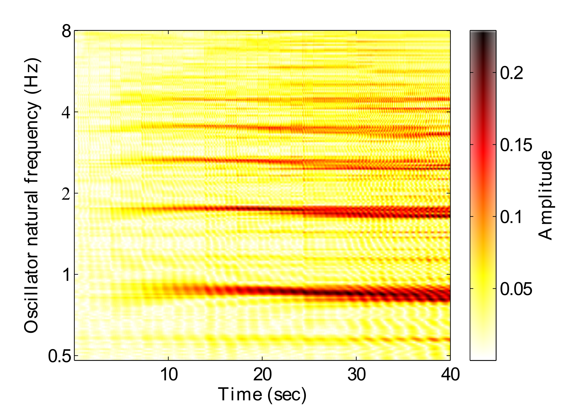
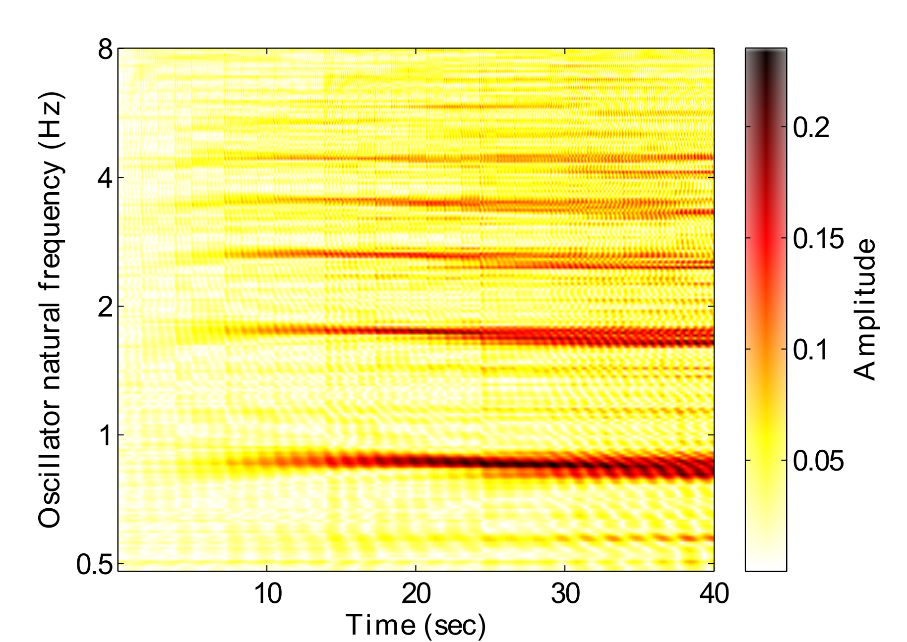
Fig. 3 shows the amplitude response of a GFNN to a rhythmic stimulus over time. Darker areas represent stronger resonances, indicating that that frequency is relevant to the music. A hierarchical structure can be seen to emerge from around 8 seconds, in relation to the pulse which is just below 2Hz in this example. At around 24 seconds, a tempo change occurs, which can be seen by the changing resonances in the figure. These resonances can be interpreted as a perception of the hierarchical metrical structure.
Velasco & Large (2011) connected two GFNNs together in a pulse detection experiment for syncopated rhythms. The two networks were modelling the sensory and motor cortices respectively. In the first network, the oscillators were set to a bifucation point between damped and spontaneous oscillation ($\alpha = 0$, $\beta_1 = −1$, $\beta_2 = −0.25$, $\delta_1 = \delta_2 = 0$ and $\epsilon = 1$). The second network was tuned to exhibit double limit cycle bifurcation behaviour ($\alpha = 0.3$, $\beta_1 = 1$, $\beta_2 = −1$, $\delta_1 = \delta_2 = 0$ and $\epsilon = 1$), allowing for greater memory and threshold properties. The first network was stimulated by a rhythmic stimulus, and the second was driven by the first. The two networks were also internally connected in integer ratio relationships such as 1:3 and 1:2, these connections were fixed and assumed to have been learned through the Hebbian process shown in Eq. (3) and Eq. (4). The results showed that the predictions of the model confirm observations in human performance, implying that the brain may be adding frequency information to a signal to infer pulse and metre (Large et al., 2015). Other rhythmic studies with GFNNs include rhythm categorisation (Bååth et al., 2013) and polyrhythmic analysis (Angelis et al., 2013).
Changes to the nonlinear resonance patterns in the GFNN over time and the learned connection matrix enables a similar analytical method to IMA’s inner structures (see Section 2.2), but is grounded more in physiology by taking an auditory approach rather than solely basing the analysis on symbolic data (the musical score).
Computationally processing an audio signal to determine pulse event onset times is termed beat tracking. It falls into a branch of Music Information Retrieval (MIR) known as automatic rhythm description (Gouyon & Dixon, 2005). Beat tracking is useful for many MIR applications, such as tempo induction, which describes the rate of the pulse (Gouyon et al., 2006); rhythm categorisation, which attempts to identify and group rhythmic patterns (Bååth et al., 2013; Dixon et al., 2004); downbeat tracking and structural segmentation, which aims to meaningfully split the audio into its musical sections such as measures and phrases (Levy et al., 2006; F. Krebs et al., 2013); and automatic transcription, which aims to convert audio data into a symbolic format (Klapuri, 2004).
Automated beat tracking has a long history of research dating back to 1990 (Allen & Dannenberg, 1990). Large used an early version of the nonlinear resonance model to track beats in performed piano music (Large, 1995). Scheirer’s (1998) system uses linear comb filters, which operate on similar principles to Large and Kolen’s early work on nonlinear resonance (Large & Kolen, 1994). The comb filter’s state is able to represent the rhythmic content directly, and can track tempo changes by only considering one metrical level. Klapuri et al.’s more recent system builds on Scheirer’s design by also using comb filters, but extends the model to three metrical levels (Klapuri et al., 2006). More recently, Böck et al. (2015) used a particular type of Recurrent Neural Network called a Long Short-Term Memory Network (LSTM). The MIR Evaluation eXchange (MIREX) project (http://www.music-ir.org/mirex/) runs a beat tracking task each year, which evaluates several submitted systems against various datasets.
State-of-the-art beat trackers do a relativity good job of finding the pulse in music with a strong beat and a steady tempo, yet we are still far from matching the human level of beat induction. Despite a recent surge in new beat-tracking systems, there has been little improvement over Klapuri et al.’s (2006) system.
Grosche et al. (2010) have performed an in-depth analysis of beat tracking failures on the Chopin Mazurka dataset (MAZ) (http://www.mazurka.org.uk/). MAZ is a collection of audio recordings comprising on average 50 performances of each of Chopin’s Mazurkas. Grosche et al. tested three beat tracking algorithms on a MAZ subset and looked for consistent failures in the algorithms’ output with the assumption that these consistent failures would indicate some musical properties that the algorithms were struggling with. They found that properties such as expressive timing and ornamental flourishes were contributing to the beat trackers’ failures.
Holzapfel et al. (2012) have selected “difficult” excerpts for a new beat tracking dataset by a selective sampling approach. Rather than compare one beat tracker’s output to some ground truth annotation, several beat trackers’ outputs were compared against each other. If there was a large amount of mutual disagreement between predicted beat locations, the track was assumed to be difficult for current algorithms, and was selected for beat annotation and inclusion in the new dataset. This resulted in a new annotated dataset, now publicly available as the SMC dataset (http://smc.inescporto.pt/research/data-2/).
The SMC excerpts are annotated with a selection of signal property descriptors. This allows for a description of what may contribute to an excerpt’s difficulty. There are several timbrel descriptors such as a lack of transient sounds, quiet accompaniment and wide dynamic range, but most of the descriptors refer to temporal aspects of the music, such as slow or varying tempo, ornamentation, and syncopation. Over half of the dataset is tagged as being expressively timed.
From this it is clear that being able to track expressive timing variations in performed music is one area in which there is much room for improvement. This is especially true if one is attempting to achieve a more human-like performance from the beat tracking algorithms. This has been attempted in many cases, most notably in the work of Dixon (2001) and Dixon & Goebl (2002). However, these systems do not perform well on today’s standard datasets, scoring poorly on the SMC dataset in 2014’s MIREX results.
As mentioned earlier, interest in musical expression goes back to the ancient Greeks and around one hundred years ago empirical research in this area started. The research field looks at what emotional meanings can be expressed in music, and what musical structures can contribute to the perception of such emotions in the listener. These structures can be made up of multi faceted musical concepts such as dynamics, tempo, articulation, and timbre. Here we focus on the temporal aspects of expression.
Performers have been shown to express the metrical structure of a piece of music by tending to slow down at the end of metrical groupings. The amount a performer slows down correlates to the importance of the metrical level boundary (Clarke, 2001). It is well known that humans can successfully identify metre and follow the tempo based off such an expressive rhythm (Epstein, 1995). Rankin et al. (2009) conducted a recent study on human beat induction and found that subjects were able to adapt to relatively large fluctuations in tempo resulting from performances of piano music in various genres. The participants could successfully find a pulse at the crotchet (quarter note) or quaver (8th note) metrical level. Skilled performers are able to accurately reproduce a variation from one performance to the next (N. Todd, 1989), and listeners are also able to perceive meaning in the deviations from the implied metrical structure (Epstein, 1995; Clarke, 1999).
According to Kirke & Miranda (2009), the introduction of built-in sequencers into synthesizers in the early 1980s contributed to a new, perfectly periodic timing, which sounded robotic to the ear. Rather than look for ways to make this timing model more human-like, artists embraced the robotic style to produce new genres of music such as synth pop and electronic dance music, which soon dominated the popular music scene.
Computer systems for expressive music performance (CSEMPs) received little attention from both academia and the industry at large. However, some research was done, such as N. Todd’s computational model of rubato (N. Todd, 1989).
One of the most common expressive devices when performing music is the use of rubato to subtly vary the tempo over a phase or an entire piece. N. Todd produced a model of rubato implemented in Lisp which is able to predict durations of events for use in synthesis.
The original model was based on Lerdahl and Jackendoff’s ideas on time span reduction in GTTM. However, this was deemed psychologically implausible as it places too high a demand on a performer’s short-term memory. In a similar way to IMA’s spectral weight, the model considers all events regardless of time differences.
N. Todd’s improved model incorporates a hierarchic model for timing units from a piece-wise global scale to beat-wise local scale. It works by looking at a score and forming an internal representation via GTTM’s grouping structures.
This internal representation is then used in a mapping function, outputting a duration structure as a list of numbers. Even though the model makes predictions about timing and rubato, it forms an analytical theory of performance rather than a prescriptive theory.
Today, research into CSEMPs is a small but important field within Computer Music. Widmer & Goebl (2004) have published an overview of existing computational models, and Kirke & Miranda (2009) have produced a survey of available CSEMPs.
P.M. Todd (1989) and Mozer (1994) were among the first to utilise a connectionist machine learning approach to music generation. This approach is advantageous over rule-based systems, which can be strict, lack novelty, and not deal with unexpected inputs very well. Instead, the structure of existing musical examples are learned by the network and generalisations are made from these learned structures to compose new pieces.
Both P.M. Todd and Mozer’s systems are recurrent networks that are trained to predict melody. They take as input the current musical context as a pitch class and note onset marker and predict the same parameters at the next time step. In this way the problem of melody modelling is simplified by removing timbre and velocity elements, and discretising the time dimension into windowed samples.
Whilst P.M. Todd and Mozer were concerned predicting melodies as pitch sequences over time, Gasser et al. (1999) have taken a connectionist approach to perceive and produce rhythms that conform to particular metres. SONOR is a self-organising neural network of adaptive oscillators that uses Hebbian learning to prefer patterns similar to those it has been exposed to in a learning phase. A single input/output (IO) node operates in two modes: perception and production. In the perception mode, the IO node is excited by patterns of strong and weak beats, conforming to a specific metre. Hebbian learning is used to create connections and between the oscillators in the network. Once these connections have been learned, the network can be switched to production mode, reproducing patterns that match the metre of the stimuli.
Recurrent neural networks (RNNs) such as the those used in the above systems can be good at learning temporal patterns, but, as noted by P.M. Todd (1989) and Mozer (1994), often lack global coherence due to the lack of long-term memory. This results in sequences with good local structures, but long-term dependencies are often lost. One way of tackling this problem is to introduce a series of time lags into the network input, so that past values of the input are presented to the network along with the present.
\begin{equation} y(t) = f(y(t-1) ... y(t-l)) \label{eq:tslag} \end{equation}Eq. (5) shows a simple time-series predictor where y represents a variable to be modelled, $t$ is time and $l$ is the number of lag steps in time. Kalos (2006) used a model of a similar type known as a Nonlinear Auto-Regression model with eXtra inputs (NARX) to generate music data in symbolic MIDI format. One advantage of this method is that it performs well on polyphonic music, but the time lag method still does not capture long-term structure very successfully.
Long Short-Term Memory Neural Networks (LSTMs) were specifically designed to overcome the problem of modelling long term structures. Hochreiter & Schmidhuber (1997) noted that whilst RNNs could theoretically learn infinitely long patterns, in practice this was difficult due to the “vanishing gradient problem” (Hochreiter & Schmidhuber, 1997). The gradient of the total output error with respect to previous inputs can quickly vanishes as the time lags between relevant inputs and errors increase. It can take as little as five time steps for this problem to occur in an RNN (Gers & Schmidhuber, 2001). In an LSTM, a self-connected node known as the Constant Error Carousel (CEC) ensures constant error flow back through time, meaning that LSTMs can bridge time lags in excess of 1,000 time steps (Hochreiter & Schmidhuber, 1997).
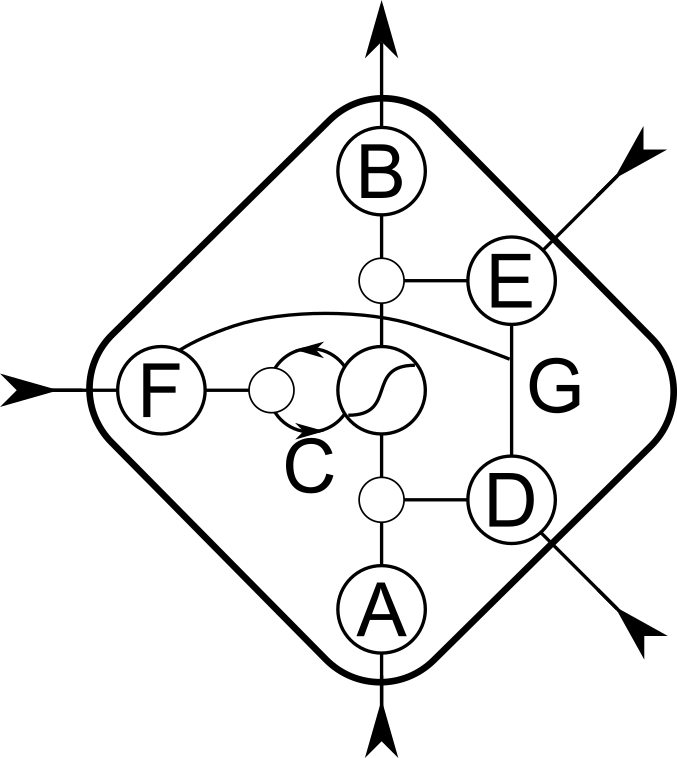
A simplified diagram of an LSTM memory block can be seen in Fig. 4. The input and output gates control how information flows into and out of the CEC, and the forget gate controls when the CEC is reset. The input, output and forget gates are connected via “peepholes”. For a full specification of the LSTM model we refer to (Hochreiter & Schmidhuber, 1997) and (Gers et al., 2000).
As time-series predictors, LSTMs perform very well, as is shown by Böck et al.’s beat tracker (2015). LSTMs have also had some success in generative systems: Eck & Schmidhuber (2002) trained LSTMs which were able to improvise chord progressions in the blues and more recently Coca et al. (2013) used LSTMs to generate melodies that fit within user specified parameters.
In our previous work, we have combined a GFNN with an LSTM (GFNN-LSTM) as two layers in an RNN chain and used it to predict melodies (Lambert et al., 2014a, 2014b). Several GFNN-LSTMs were trained on a corpus of monophonic symbolic folk music from the Essen Folksong Collection (Schaffrath, 1995).
In the first set of experiments, the networks were trained to predict the next pitch in metrically-quantised time-series data. A single output was used to predict the scale degree of the next sample in the data, which was sampled such that one sample was equivalent to a semiquaver (16th note). The second set of experiments modelled both pitch and rhythm with two outputs from the GFNN-LSTM: the first one being identical to the earlier experiment, and the second was trained to predict the rhythmic onset pattern used to stimulate the GFNN. The resolution of the time series was also increased by a factor of two, such that each sample corresponded to a demisemiquaver (32nd note).
Our overall results of these two experiments showed that providing nonlinear resonance data from the GFNN helped to improve melody prediction with an LSTM. We hypothesise that this is due to the LSTM being able to make use of the relatively long temporal resonance in the GFNN output, and therefore model more coherent long-term structures. In all cases GFNNs improved the performance of pitch and onset prediction.
Our previous results from initial experimentation (Lambert et al., 2014a, 2014b) gave some indication that better melody models can be created by modelling metrical structures with a GFNN.
The system we present here is a significant step beyond our previous work. For the first time we are dealing with audio data, which opens the system up for a much wider set of live and off-line applications, but comes with its own set of new problems to solve. We are now using data at varying tempos and sampled at an arbitrary sample rate, not one that is metrically quantised as per our pervious work. Furthermore, we are for the first time experimenting with enabling Hebbian learning within the GFNN in the hope this will enable stronger metric hierarchies and faster entrainment responses to emerge from the nonlinear resonance.
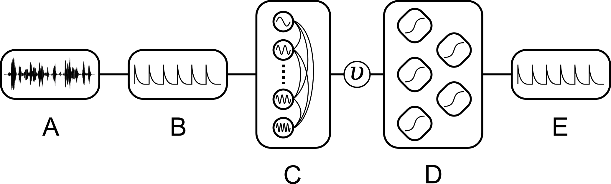
The aim of this experiment was to train a GFNN-LSTM to predict expressive rhythmic events. The system takes audio data as input and outputs an event activation function. The system operates in a number of stages which are detailed below. A schematic of the system is provided in Fig. 5.
We used a subset of MAZ, since pieces themselves are expressively performed by the various performers and vary in tempo and dynamics throughout the performance. However, the pieces are all within the same genre and are all performed on the piano, making drawing conclusions about the rhythmic aspects more valid. We have made a subset of 50 excerpts, each 40 seconds long, by randomly choosing annotated excerpts of full pieces and slicing 40 seconds worth of data.
When processing audio data for rhythmic events, it is common to first transform the audio signal into a more rhythmically meaningful representation from which these events can be inferred. This representation could be extracted note onsets in binary form, or a continuous function that exhibits peaks at likely onset locations (Scheirer, 1998). These functions are called onset detection functions and their outputs are known as mid-level representations.
Since we are dealing with expressively rich audio, we have chosen an onset detection function which is sensitive both to sharp and soft attack events such as those found in the MAZ piano performances. From Bello et al.’s (2005) tutorial on onset detection in music signals, we have selected the complex spectral difference (CSD) onset detection function. This detection function emphasises note onsets by analysing the extent to which the spectral properties of the signal at the onset of musical events are changing. The function operates in complex domain of a frequency spectrum where note onsets are predicted to occur a result of significant changes in the magnitude and/or phase spectra. By considering both magnitude and phase spectra, CSD can capture soft changes in pitch and hard rhythmic events.
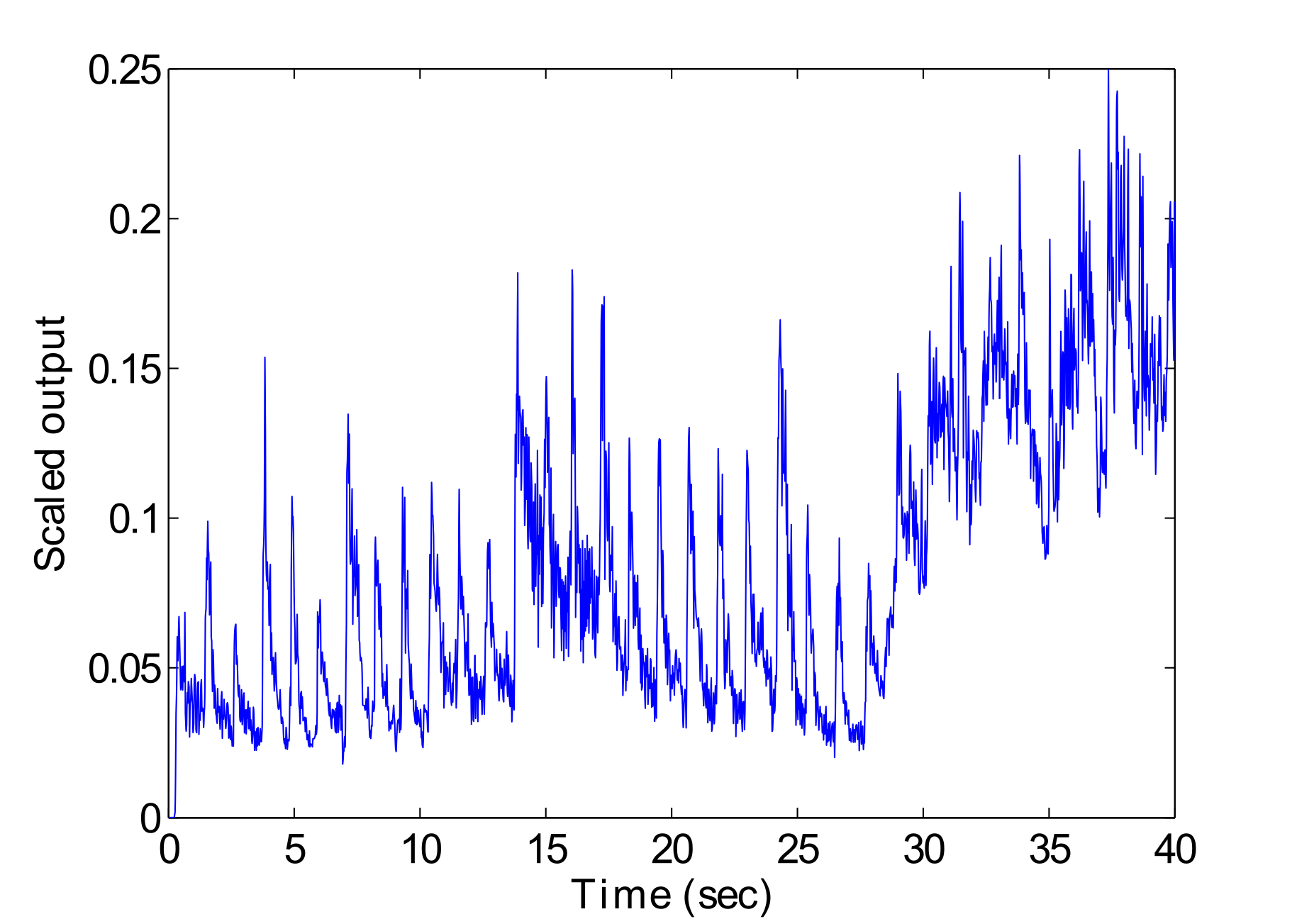
Fig. 6 displays an example output of CSD. Here the output range has been scaled to a 0 to 0.25 scale for input into the GFNN. This continuous function output can be converted into binary onset data by using suitable threshold levels for peak picking. A sample rate of 86.025Hz was used, which was recently found to yield accurate detection results (Davies & Plumbley, 2007).
The GFNN was implemented in MATLAB using the GrFNN Toolbox (Large et al., 2014). It consisted of 192 oscillators, logarithmically distributed with natural frequencies in a rhythmic range of 0.5Hz to 8Hz. The GFNN was stimulated by rhythmic time-series data in the form of the mid-level representation of the audio data.
We have selected two parameter sets for the oscillators themselves, obtained from the examples in the GrFNN Toolbox. These different parameters affect the way the oscillators behave. The first parameter set puts the oscillator at the bifurcation point between damped and spontaneous oscillation. We term this “critical mode”, as the oscillator resonates with input, but the amplitude slowly decays over time in the absence of input: $\alpha = 0$, $\beta_1 = \beta_2 = -1$, $\delta_1 = \delta_2 = 0$, $\epsilon = 1$. By setting $\delta_1 = 1$, we define the second parameter set: “detune mode”. $\delta_1$ affects the imaginary plane only, which is the oscillators inhibitor. This allows the oscillator to change its natural frequency more freely, especially in response to strong stimuli. As a result, this could allow for improved tracking of tempo changes.
We have also selected three approaches to performing the Hebbian learning in the GFNN layer. The first approach simply has no connectivity between oscillators and therefore no learning activated at all. This is so that we can measure the effect (if any) that learning in the GFNN layer has on the overall predictions of the system.
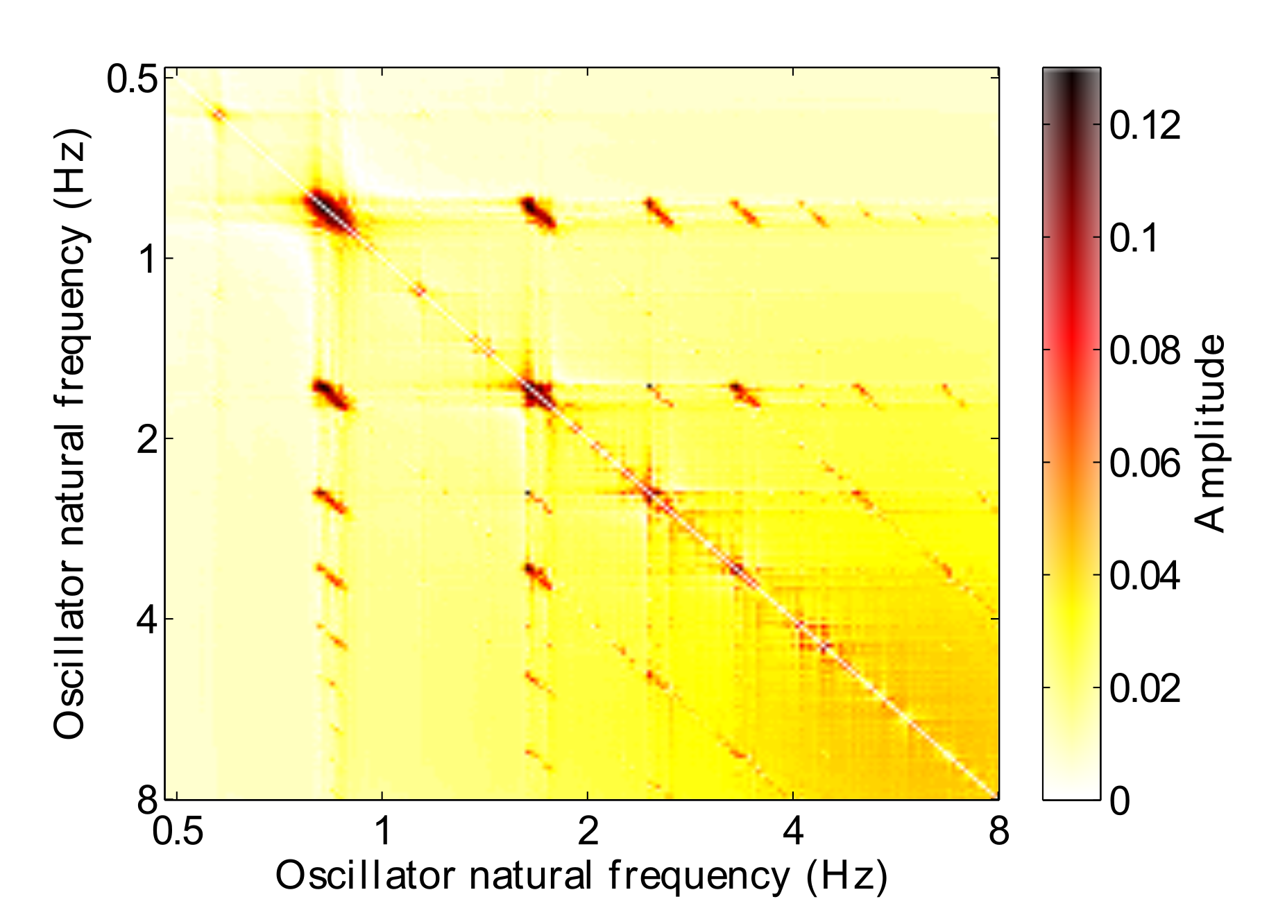
The second approach is to activate online Hebbian learning with the following parameters: $\lambda = 0$, $\mu_1 = -1$, $\mu_2 = -50$, $\epsilon_c = 4$ and $\kappa = 1$. Under these parameters, the network should learn connections between related frequencies as they resonate to the stimulus. Fig. 7 shows an example connection matrix that is learned from one particular excerpt. Taken together, the behaviour of the GFNN over time and the learned connection matrix enables a similar analytical method to IMA (see Section 2.2), but is a continuous-time model, whereas IMA uses discrete, metrically quantised time steps.
From Fig. 7 we can see that high order hierarchical relationships have been learned by the oscillators. However, these relationships are only valid for the particular excerpt that they have been learned with: they are localised to specific fixed frequencies rather than being a generalisation. This has both positive and negative aspects. On the positive side, we can use the connection matrix as a way of analysing the frequency responses of the network. However, applying this this connection matrix in a prediction task would not be that useful, as any rhythm outside this particular tempo with different local metres would not exhibit predictable behaviour.
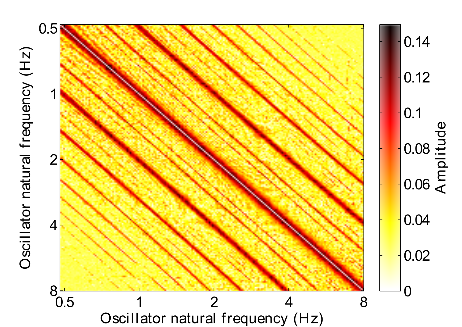
By activating the learning rule when the oscillators are set to operate in limit cycle mode (a spontaneous oscillation in the absence of input), the internal connections can be learned in the absence of any stimulus. The resulting connectivity matrix is shown in Fig. 8. This provides a much more general state for the connection matrix to be in and potentially overcomes the limitations of the fixed frequency connections learned in Fig. 7.
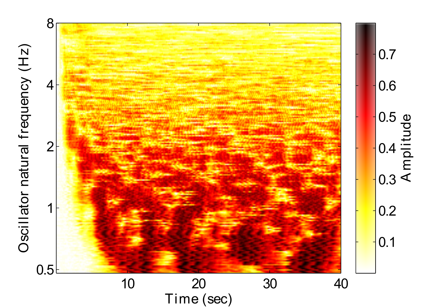
However, we can see in the network response (Fig. 9) that fixing the connections at this state results in a much noisier output of the GFNN. Resonances do build up very quickly, but the resulting oscillator output does not resemble the structured hierarchy found in Fig. 3. Essentially there are too many connections in the GFNN, leading to a “cascade” effect where a strong resonant response to the stimulus is transferred down the frequency gradient in a wave. This amounts to a GFNN output which is to noisy to be used for any subsequent machine learning tasks.
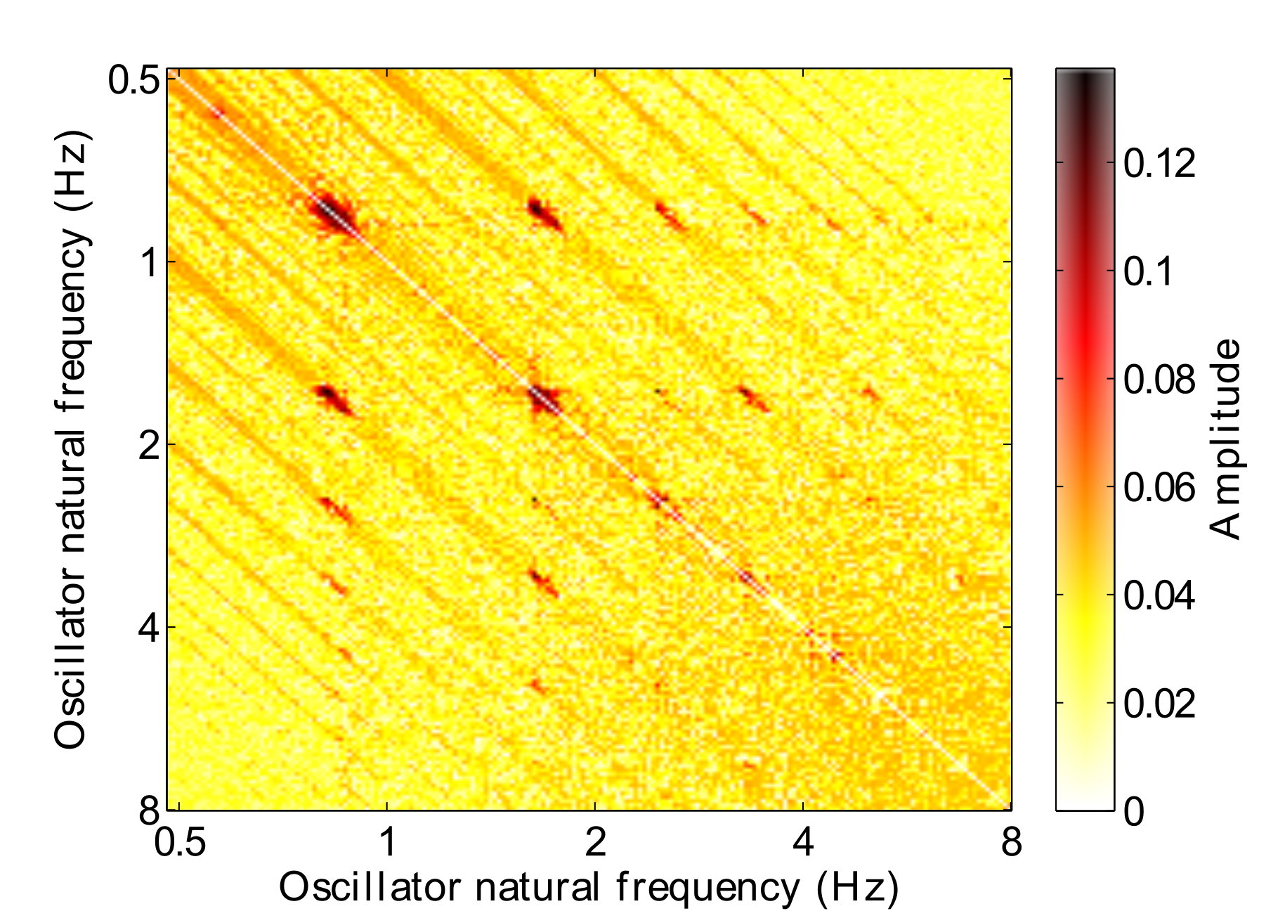
This can be counteracted by keeping online learning activated and also setting the initial connectivity state with that learned in limit cycle mode. The resulting connectivity matrix can be seen in Fig. 10. The matrix exhibits strong local connections at frequencies specific to the excerpt, but more general high order connections are still present in the matrix. The amplitude response of the network (Fig. 11) shows a clear hierarchy of frequencies whilst also displaying a fast resonance response and less noise. This is the third approach to Hebbian learning we have taken in this paper and we term it “InitOnline”.
We found in some initial experimentation that with Hebbian learning activated, the differential equations that drive the connectivity matrix can become unstable and result in an infinite magnitude. To ensure greater stability in the system, we have limited the connections in the connectivity matrix to have a magnitude less than $[\frac{1}{\sqrt{\epsilon_c}}]$ (0.5 in our experiments). We also and rescaled all stimuli to be in the range $0 <= x(t) <= 0.25$.
The LSTM was implemented in Python using the PyBrain library (Schaul et al., 2010). For each variation of the GFNN, we trained two LSTM topologies. The first had 192 linear inputs, one for each oscillator in the GFNN, which took the real part of each oscillator’s output. We term this the “Full” LSTM. The real part of the canonical oscillation is a representation of excitatory neural population; by discarding the imaginary part, we still retain a meaningful representation of the oscillation, but increase the simplicity of the input to the LSTM (Large et al., 2015). The second topology took only one linear input, which consisted of the mean field of the real-valued GFNN. The mean field reduces the dimensionality of the input whilst retaining frequency information within the signal. We term this the “Mean” LSTM.
All networks used the standard LSTM model with peephole connections enabled. The number of hidden LSTM blocks in the hidden layer was fixed at 10, with full recurrent connections. The number of blocks was chosen based on previous results which found it to provide reasonable prediction accuracy, whilst minimising the computational complexity of the LSTM (Lambert et al., 2014b).
All networks had one single linear output, which serves as a rhythmic event predictor. The target data used was the output of the onset detection algorithm, where the samples were shifted so that the network was predicting what should happen next. The input and target data was normalised before training.
Training was done by backpropagation through time (Werbos, 1990) using RProp- (Igel & Hüsken, 2000). During training we used k-fold crossvalidation (Kohavi, 1995). In $k$-fold cross validation, the dataset is divided into $k$ equal parts, or “folds”. A single fold is retained as the “validation data” and is used for parameter optimisation, and the remaining $k - 1$ folds are used as training data. The cross-validation process is then repeated $k$ times, with each of the $k$ folds used exactly once as the test data. This results in $k$ trained networks which are all evaluated on data unseen to the network during the training phase. For our experiments $k$ was fixed at 5, and a maximum of 350 training epochs was set per fold. Training stopped when the total error had not improved for 20 epochs, or when this limit was reached, whichever came sooner.
This experiment was designed to discover if the GFNN-LSTM is able to make good predictions in terms of the rhythmic structure. Therefore we are evaluating the system on its ability to predict expressively timed rhythmic events, whilst varying the parameters of the GFNN and connectivity. We are not explicitly evaluating the system’s production of expressive timing itself, but we are implicitly evaluating the tracking and representation of expressive timing, as it is reasonable to assume that a meaningful internal representation of metrical structure is needed for accurate predictions.
The results have been evaluated using several metrics. The first three results refer to the binary prediction of rhythmic events of pitch changes using the standard information retrieval metrics of precision, recall and F-measure, where higher values are better. Events are predicted using a gradient threshold of the output data. The threshold looks for peaks in the signal by tracking gradient changes from positive to negative. When this gradient change occurs, an onset has taken place and is recorded as such.
These events were subject to a tolerance window of ±58.1ms. This means that an onset can occur within this time window and still be deemed a true positive. At the sample rate used in this experiment, this equates to 5 samples either side of an event. We also insured that neither the target nor the output can have onsets faster than a rate of 16Hz, which is largely considered to be the limit of where rhythm starts to be perceived as pitch (Large, 2010). These are limitations to our evaluation method, but since we are mainly interested in predicted rhythmic structures and are not explicitly evaluating the production of expressive micro-timing, we believe they are acceptable concessions.
We have also provided the mean squared error (MSE) and the Pearson product-moment correlation coefficient (PCC) of the output signals, which provide overall similarity measures.
For all metrics the first 5 seconds of output by the network are ignored, making the evaluation only on the final 35 seconds of predictions.
Tab. 1 and Tab. 2 display the results of the experiment, and Fig. 12 to Fig. 17 show examples of each network’s output. These numerical metrics and visual figures provide some indication of how well the system is capturing the rhythmic structures. However, this information may be better understood by listening to the predicted rhythms. To this end, the reader is invited to visit this paper’s accompanying website (http://andyroid.co.uk/research/gfnn_lstm_rhythm_prediction), where we have assembled a collection of audio examples for each network’s target and output data.


Our best overall GFNN-LSTM for expressive rhythm prediction incorporates detune oscillators, online learning with initial generic connections in the GFNN layer, and mean field connections.
We can see from the results that the mean field networks always outperformed the GFNN-LSTM with a full connection. This could be due to the mean field being able to capture the most resonant frequencies, whilst filtering out the noise of some less resonant frequencies. The resulting signal to the LSTM would therefore be more relevant for predicting rhythmic events. However, this may also be due to the limited number of LSTM blocks in each network forming a bottleneck in the fully connected networks. Increasing number of hidden LSTM blocks may mitigate this limitation.
One downside of the mean field networks is that drastically reducing the dimensionality in this way could cause some over-fitting. We can see in the results that whist performance improved in all cases using the mean field, the standard deviation also increased. This means there was a greater range of performances between the folds and could possibly indicate some networks being trained to local optima. During training we observed that the mean field networks took many more epochs for errors to converge. This could possibly be addressed by using sub-band mean fields, or some other method to reduce the dimensionality between layers.
In all cases, the detune oscillators outperformed the critical oscillators. In most cases the standard deviation was also decreased by using detune oscillators. This can be attributed to the greater amount of change in the imaginary part of the oscillator (inhibitory neural population). Tempo changes can be tracked as an entrainment process between a local population of oscillators in the network. Where there is a local area of strong resonance the oscillators will take on very near frequencies to one another. As the stimulus frequency changes, this local area will be able to follow it, moving the local resonance area along the frequency gradient.
It is interesting to note that applying online learning to the network did improve the overall MSE of the signal, but the F-measure actually performed worse in all cases. Perhaps an adaptive threshold may be the solution to this problem, as the GFNN signal changes in response to previous inputs and the connections begin to form.
In our previous work on rhythm prediction with the GFNN-LSTM model (Lambert et al., 2014b), the best network achieved a rhythm prediction mean F-measure of 82.2%. Comparing this with the 71.8% mean achieved here may at first seem a little underwhelming. However, these new results represent a significant change in the signal input, and reflects the added difficulty of the task. Our previous work was on symbolic music at a fixed tempo and without expressive variation, whereas this study is undertaken on audio data performed in an expressive way. The overall best single fold (Detune oscillators, InitOnline connections, and Mean input) was achieving an F-measure of 77.2%, which we believe is extremely promising.
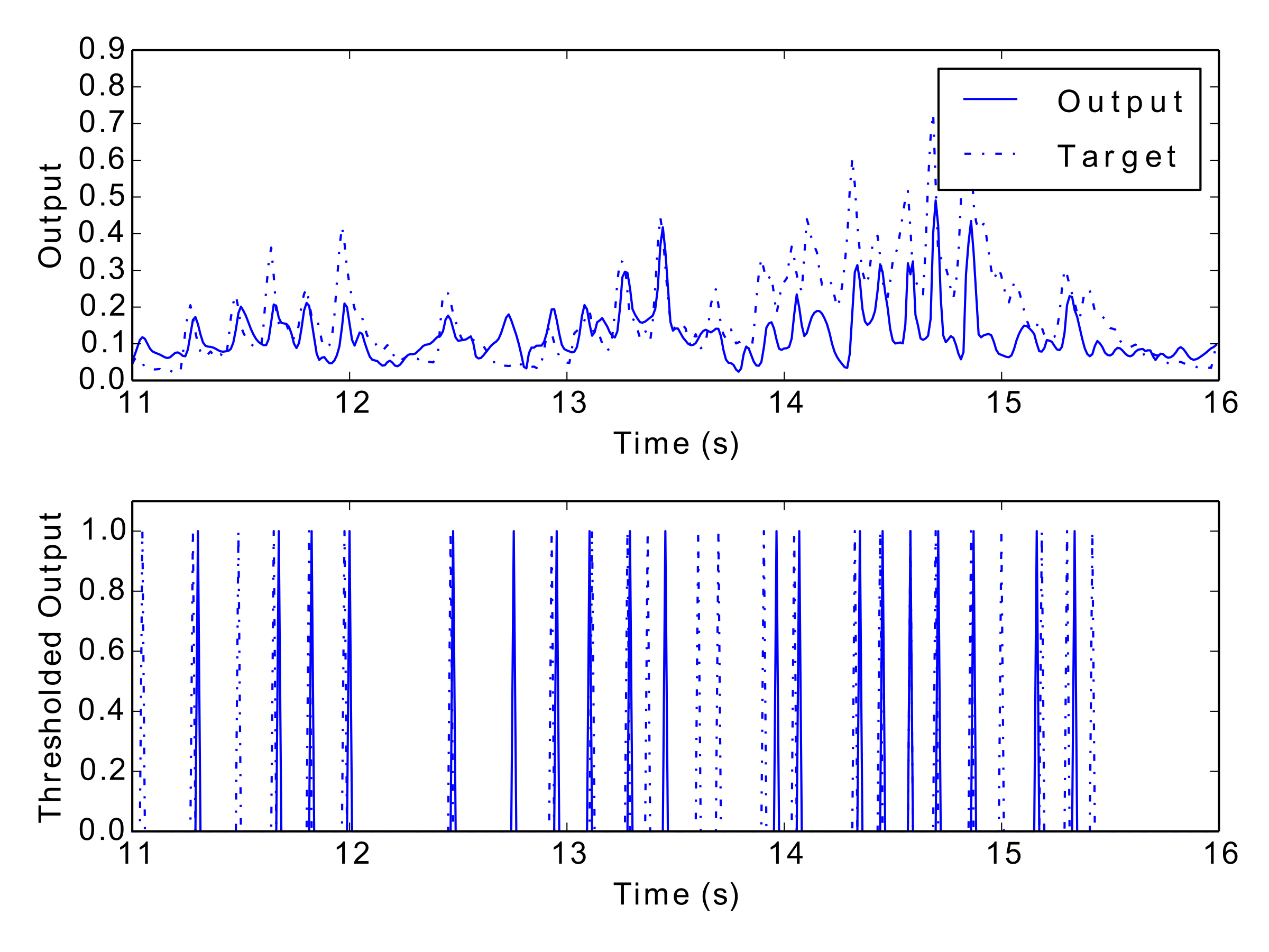
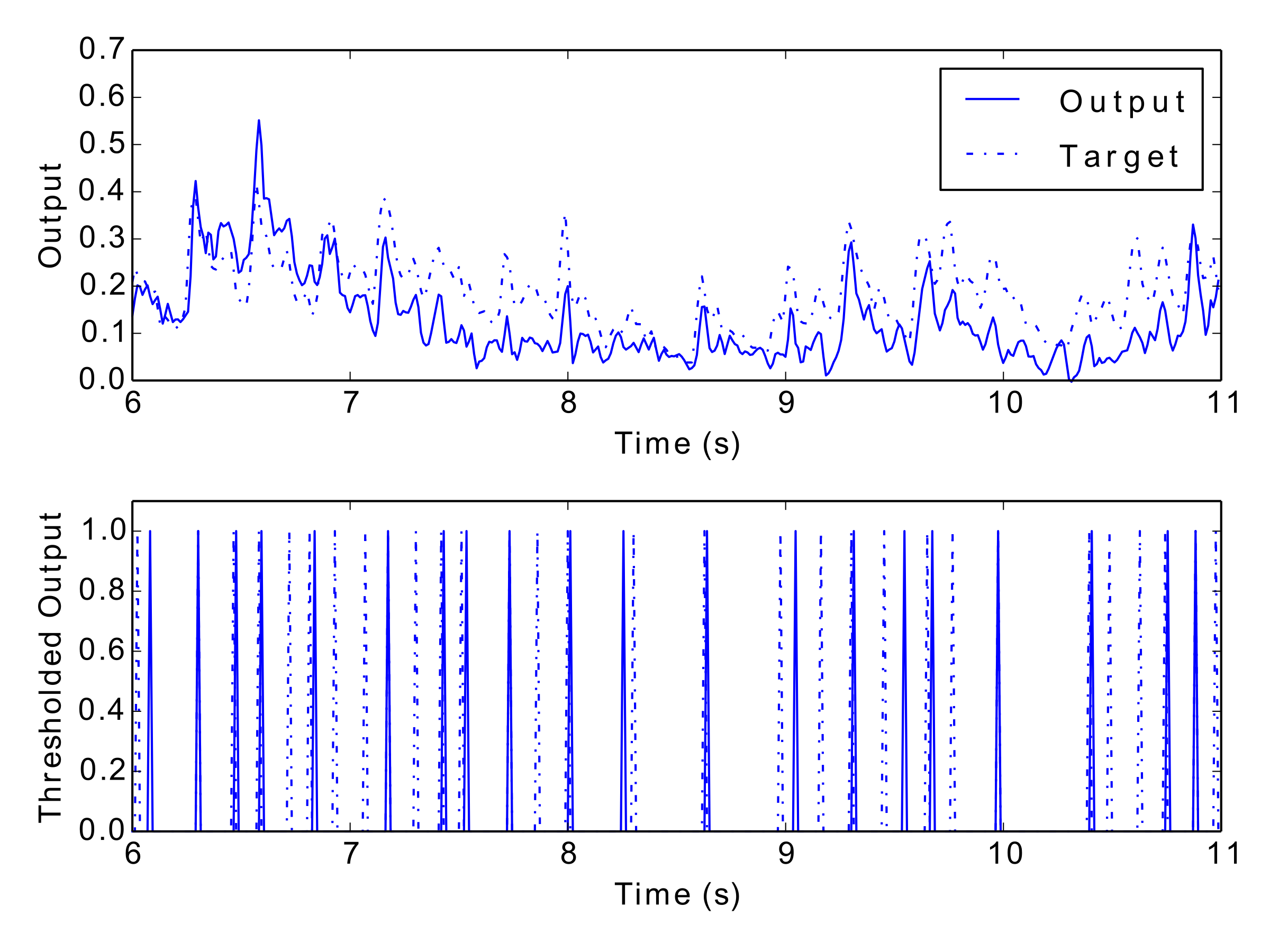
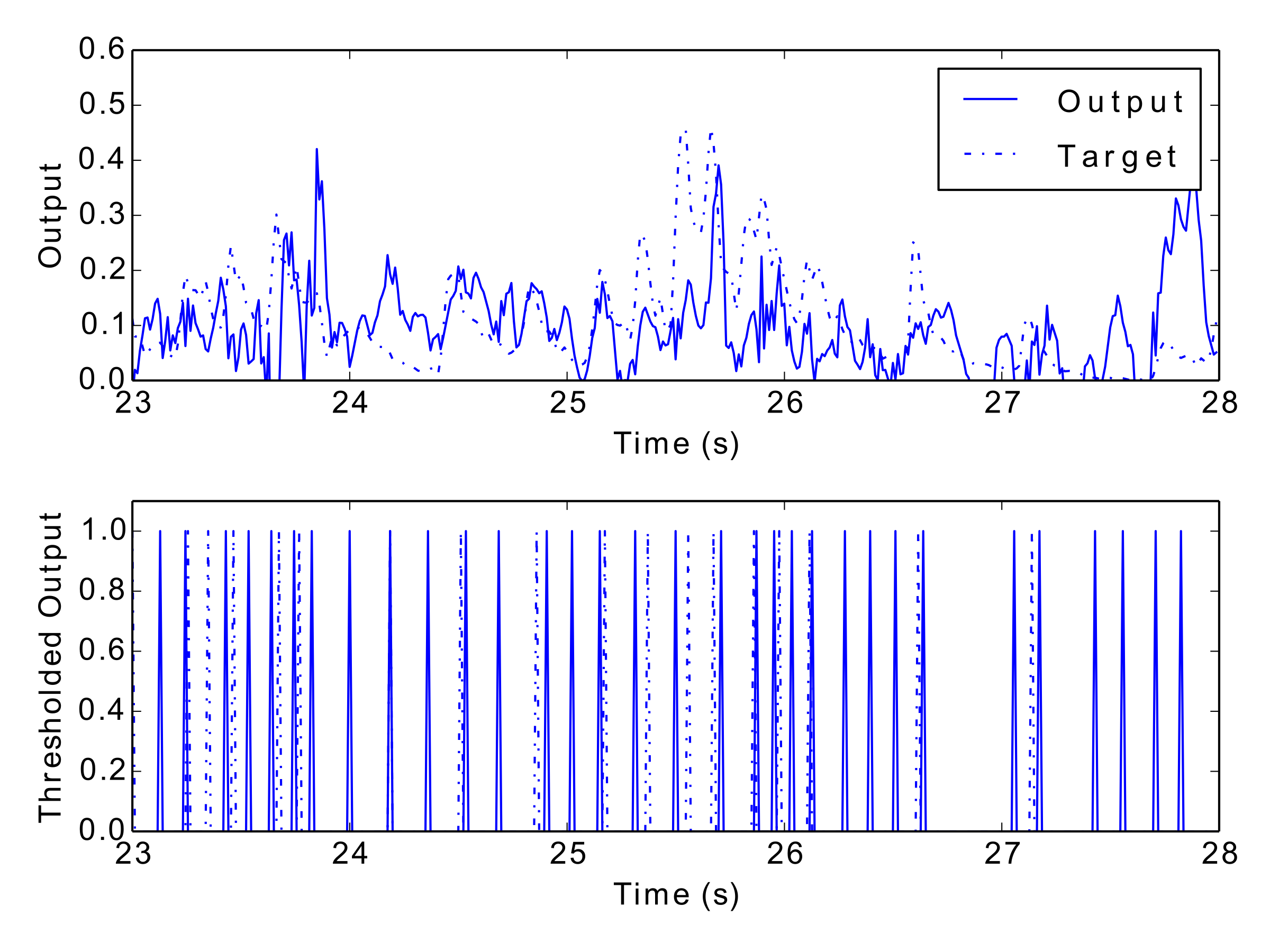

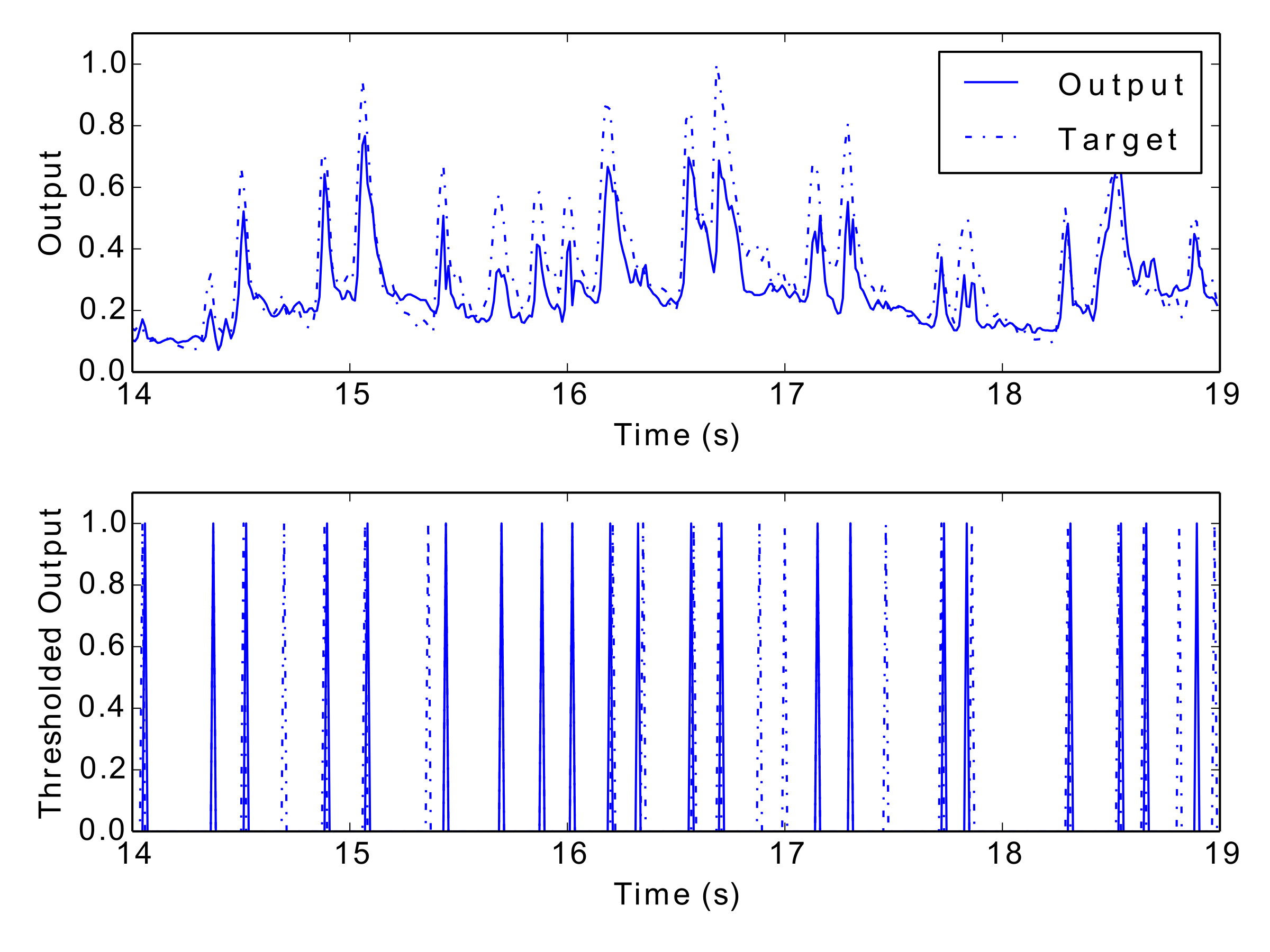
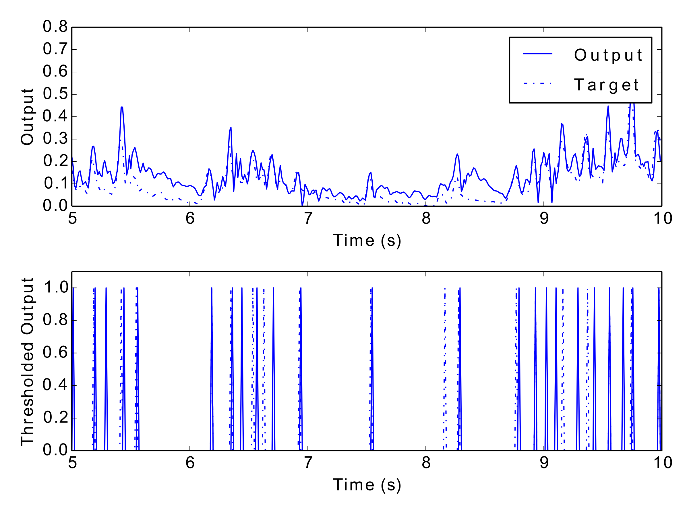
Figs 12–17: Example outputs from various trained networks over time. The top part of each figure shows the continuous output set against the training data, whereas the bottom part shows extracted events after a threshold has been applied.
Our approach to rhythm prediction is a novel one, which makes a comparative statement difficult to make. However, we can draw similarities between our system and an MIR beat tracker; both are processing audio systems to extract rhythmic predictions. The best MIREX beat tracker in 2015 scored an F-measure of 74.2% (see (Böck et al., 2015)) on the same dataset used above. This system has a similar design to the GFNN-LSTM: spectrogram change information is input into an LSTM which, is trained to predict beat events. These predictions are processed with a bank of resonating comb filters to help smooth the output. Whilst we cannot make a direct comparison as we are predicting expressive rhythm events not pulse events, we believe a comparison with this system is helpful for two reasons. Firstly it shows a similar method is producing state-of-the-art results in a field where comparisons are easier to make, and secondly it hints that our system is performing well on this dataset.
Our system takes audio data as input and outputs a new rhythm prediction signal. The rhythm output can be easily used to produce a new audio signal and exciting the network with untrained data will produce novel outputs. We therefore label this application of a GFNN-LSTM as an expressive rhythm generative system.
It would be trivial to close the loop in our system, creating a feedback between input and output. This would allow indefinite, self-driven generation of new rhythmic structures which can be evaluated for their novelty.
When considering generative software, validating the work both in terms of the computational system and the output it creates is still a challenge for the community at large. The way these systems and their outputs can be compared and evaluated is an ongoing problem facing the computational creativity community (Jordanous, 2011).
Adopting Jordanous’ (2012) Standardised Procedure for Evaluating Creative Systems (SPECS) methodology, we make the following statements about our system as it stands, as a generative system:
Eigenfeldt et al. (2013) have also contributed towards a solution to the evaluation problem by proposing a music metacreation (MUME) taxonomy to facilitate discussions around measuring metacreative systems and works. The taxonomy is based around the agency or autonomy of the system in question, since in MUME the computational system is an active creative agent. By focusing on the system’s autonomy, one is able to distinguish between the composer’s (system designer’s) influence on the system and the performance elements, which may change from execution to execution. The MUME taxonomy places the metacreation of the system on a gradient through the following seven levels of creative autonomy:
We believe our system exhibits all of the features up to level 5 in this taxonomy. The gestural style is determined my the training data, which in our case is MAZ, and is unable to produce rhythms in any other style.
In this paper we have detailed a multi-layered recurrent neural network model for expressively timed rhythmic perception, prediction and production. The model consists of a perception layer, provided by a GFNN, and a prediction layer provided by an LSTM. Production is be achieved by creating a feedback loop between input and output. We have evaluated the GFNN-LSTM on a dataset selected for its expressive timing qualities and found it to perform at a comparable standard to a previous experiment undertaken on symbolic data.
Our system’s performance is comparable to state-of-the-art beat tracking systems. For the purposes of rhythm generation, we feel that the F-measure results reported here are already in a good range. Greater values may lead to too predictable and repetitive rhythms, lacking in the novelty expected in human expressive music. On the other hand, lower values may make the generated rhythms too random and irregular, so that they may even not be perceived as rhythmic at all. To make any firm conclusions on this, we would need to conduct formal listening tests based on the rhythms we have generated with our system. This is left for future work.
Another interesting avenue for future analysis is to explicitly evaluate the system’s production of expressive timing. To achieve this we will possibly need to remove the tolerance window and analyse time differences between the target and output events with a steady idealised pulse.
By using an oscillator network to track the metrical structure of expressively timed audio data, we are able to process the metrical structures of audio signals in real-time. We intend to extend this initial system for complete use as a generative music system. Firstly, we will incorporate polyphonic rhythms into the system, instead of outputting a single rhythm output. Secondly, incorporating some melody model as in our previous work would be of use for complete autonomy of the system as a musical agent. This would allow indefinite generation of new rhythmic and melodic structures which can be evaluated for their novelty. In doing so we will have created an expressive, generative, and autonomous real-time agent.
Many thanks to Alvaro Correia, Julien Krywyk and Jean-Baptiste Rémy for helping to curate the audio examples.
Andrew J. Elmsley (né Lambert) is supported by a PhD studentship from City University London.
There are no notes.