Stylistic composition has long been the province of aspiring composers, who might for instance (a) harmonise a given melody; (b) write one or more parts above a given bass line; or (c) compose a complete musical texture (excerpt or whole piece) in an attempt to imitate and so internalise the style of earlier masters (Gjerdingen, 2007). Algorithmic approaches to stylistic composition, such as musical dice games, predate digital music computing by two centuries (Hedges, 1978), but now the former are outweighed vastly by computational algorithmic methods (for detailed reviews, see Collins, Laney, Willis & Garthwaite, 2016; Fernández & Vico, 2013; and Niehaus, 2009). Commonly mentioned shortcomings of these computational approaches to stylistic composition are that researchers have:
Fixated on task (a), harmonisation, particularly chorale harmonisation in the style of J.S. Bach (1685–1750), at the expense of (b) or especially (c) – generating all the notes that contribute to a complete musical texture (Whorley, Wiggins, Rhodes & Pearce, 2013).
Not devised generation processes that balance small-scale, event-to-event transitions with large-scale considerations of repetitive or phrasal structure. For instance, in summarising shortcomings and establishing challenges for the field of music computing, Widmer (2016) observes that almost all models (both analytic and compositional).
“are either of a Markovian kind, assuming a strictly limited range of dependency of the musical present on the musical past … or have a kind of decaying memory (as in simple Recurrent Neural Networks). On the other hand, it is clear that music is of a fundamentally non-Markovian nature. Music is full of long-term dependencies: most pieces start and end in the same key, even if they modulate to other tonalities in between; themes return at regular or irregular intervals, after some intermittent material … What is needed, first of all, is to broadly acknowledge the non-Markovian nature of music and be critically aware of the fundamental limitations of HMMs and similar models in describing music … Second, we need more research on complex temporal models with variable degrees of memory” (p. 4).
Not, on the whole, conducted listening studies in which less or more expert participants judge and/or comment on the stylistic success of music-generating systems’ outputs (exceptions are Collins et al., 2016; Pearce & Wiggins, 2001; Pearce & Wiggins, 2007; for further discussion see Pearce, Meredith & Wiggins, 2002).
The main purpose of this article is to describe and evaluate an algorithm for stylistic composition called Racchmaninof-Jun2015, referred to hereafter as Racchmaninof, that addresses point 2 above – what we might call Widmer’s long-term dependency challenge. Rather than broadly reject the Markovian approach to modelling music, as Widmer (2016) suggests doing, we nest a Markovian approach within processes designed to ensure that the generated material has both long-term repetitive and phrasal structure. The listening study we conducted and describe below, which focused on evaluating the algorithm’s ability to generate passages in two target styles, goes some way towards addressing point 3 above – the current lack of rigorous evaluation in the field. The two target styles are four-part hymns from the Baroque era in the style of Bach and mazurkas from the Romantic era in the style of Frédéric Chopin (1810–1849). It is important to emphasise that at all times we are undertaking task (c), generating the complete musical texture, not generating melody-only material nor harmonising given melodies. In so doing, this work also contributes to redressing the imbalance highlighted in point 1.
The remainder of this article is structured as follows. A review of related work is followed by a description of the Racchmaninof algorithm, using some generated passages as concrete examples of long-term repetitive and phrasal structure. Next, we evaluate the algorithm’s output by describing the setup and results of a listening study. Finally we discuss the results of this study and the wider ramifications for the field.
Herremans & Sörensen (2013) generate fifth species counterpoint using a variable neighbourhood search (VNS) algorithm. VNS (Mladenovic & Hansen, 1997) starts from an initial random solution and searches local neighbourhoods based on small changes. Local optima are escaped through a perturbation strategy, which makes bigger changes. They exploit the formal rules of species counterpoint in order to construct an objective function to guide the search. Evaluation is informal. The approach is extended (Herremans & Sörensen, 2015) to generate contrapuntal music in the style of Bach, Haydn or Beethoven, with the incorporation of a logistical regression function (trained on a corpus) into the objective function used. Whilst optimal parameters for the VNS are selected using a statistical analysis, aesthetic judgement of the output music is based on informal reflections of the authors. In preparation for this article, we noted that the Fux application, which serves as an implementation of the above-mentioned work, is no longer accessible. Herremans, Weisser, Sörensen & Conklin (2015) combine The VNS approach with the use of first-order Markov models, which are used in the generation of objective functions. The system was used to generate bagana music, which was evaluated by an expert, who found one piece to be very good.
Whorley et al., (2013) focus on the problem of generating four-part polyphony given an existing soprano line, using multiple viewpoints (Conklin & Witten, 1995). In this work the voices are generated sequentially – first the bass, then each of the other voices. They observe that random sampling of a Markov model can lead to stylistic failure due to the selection of unlikely events and mitigate against this by imposing thresholds on the probabilities of selected events. This research extends previous efforts involving the use of viewpoints (numerical sequences that can be defined according to various dimensions of symbolically encoded music) to generate music (Conklin, 2003; Conklin & Witten, 1995). Recently, Conklin & Bigo (2015) have turned their attention to the generation of trance music via musical transformations and Cherla et al. (2013) have explored the possibility of using restricted Boltzmann machines (RBM) for melodic prediction. This latter paper is part of a wider effort to model musical style via the use of neural networks (e.g., Lattner, Grachten, & Widmer, 2016; Sturm et al., 2015). Most of the above work on viewpoints is evaluated by defining a metric according to which the output is assessed.
There is some overlap between these authors and those who in the previous decade called for and conducted evaluations via listening studies (Pearce & Wiggins, 2001; Pearce & Wiggins, 2007; Pearce, Meredith & Wiggins, 2002). Amabile’s (1996) Consensual Assessment Technique (CAT) was adapted from evaluation of non-musical creative products to use with music excerpts; some human-composed, some computer-generated; and a case was made for collecting listener ratings of the stylistic success of excerpts, on the grounds that this was more informative than only collecting judgements about whether a particular excerpt was perceived as human-composed or computer-generated (the latter has been referred to as a musical Turing test, Ariza, 2009; Pearce & Wiggins, 2007; Turing, 1950).
Markov-based approaches with constraints have proved a popular approach for generating music (Eigenfeldt & Pasquier, 2010; Maxwell, Eigenfeldt, Pasquier & Gonzalez Thomas, 2012). These have been posed as constraint satisfaction problems (Anders & Miranda, 2010; Papadopoulos, Pachet, Roy, & Sakellariou, 2015; Pachet & Roy, 2011) and applied to tasks such as melody generation, chord sequence generation (Pachet & Roy, 2011), accompaniment (Cont, Dubnov & Assayag, 2007) and harmonisation (Hedges, Pierre & Pachet, 2014; Pachet & Roy, 2014). The computer is generating part, but not all, of a complete musical texture. Naturally, one day such parts may be combined to form a complete musical texture. Evaluation tends to be informal: “it can be said that the musical quality is high, compared to previous approaches in automatic harmonisation” (Pachet & Roy, 2014, p. 7).
Continuing this review of Markov-based approaches with constraints, a somewhat controversial figure in the field of computer-generated music is Cope (1996, 2001, 2005) and his system Experiments in Musical Intelligence (EMI). The controversy stems in part from the feats of stylistic success that EMI apparently achieved, generating fully-fledged mazurkas in the style of Chopin and operas in the style Mozart while contemporary researchers were (and still are) communicating more modest advances in terms of generating chorale harmonisations (Ebcioğlu, 1992) or short melodies (Conklin & Witten, 1995). The lack of (a) availability of EMI’s full source code and (b) rigorous evaluation of output via expert listeners did not (and does not) necessarily demarcate Cope’s (1996, 2001, 2005) research as overly informal or unscientific, given that similar deficiencies could be highlighted with regards to much of the research cited above, but EMI’s reported successes attracted increased scrutiny and criticism (Handelman, 2005; Wiggins, 2008). These authors questioned whether a plethora of historically informed, thought-provoking, yet often quite vague descriptions of EMI, accompanying code for constituent or simpler related algorithms and YouTube videos could be accepted as evidence that the biggest challenges in simulating musical creativity had been solved.(1) We included EMI output in a listening study (Collins et al., 2016) and showed it was indistinguishable, both in terms of stylistic success ratings and binary human-composed versus computer-generated choices, from original Chopin mazurkas. We also conducted an indepth analysis of EMI output, showing that in at least one case, a twenty-bar EMI-generated passage could be transposed so that it shares 63% of notes (145 out of 230) with an existing work (the Mazurka in F minor op. 68 no. 4 by Chopin). In the context of generating a “new” work in a target style – not in the broader context of music history, where a variety of borrowing norms have prevailed (Burkholder, 2001) – it is safe to say that 63% note overlap with twenty bars of an existing work is the wrong side of the threshold for too much copying, even though the exact value of such a threshold may be difficult to determine in general (Pachet & Roy, 2014). Overall, we find two sections of Cope’s work particularly useful: the description of a formation of a Markov model over polyphonic (in the widest sense of the term) music data (Cope, 2005, p. 89) and Hofstader’s (writing in Cope, 2001) description of templagiarism, which is the process whereby abstract information about the locations of repeated sections and themes is lifted (plagiarised) from an existing piece (template, hence templagiarism) and used to guide the generation of a new passage in the target style. An example of our implementation of this process is discussed in the next section.
This review has research into “offline” systems for generating music as its focus; by which we mean that the corpus is defined and algorithms take an arbitrary amount of time, without further human intervention, to generate material – but there is work on online or interactive systems that are also intended to generate stylistic output (e.g., Nika et al., 2015). Some of these interactive systems involve embedding an offline but suitably fast generation algorithm in a user-computer feedback loop and so the embedded algorithms are another potential source of relevant work on generating stylistic material.
One could look back further than the current review and find more related work on algorithms for the generation of stylistic compositions, with the dedicated reviews or substantial review sections of Cope (1996), Fernández and Vico (2013), Nierhaus (2009) and Collins et al. (2016) providing useful starting points. Compared with earlier publications in the field of music computing, bibliographies of contemporary journal and conference papers appear to be losing touch with historical, pre-digital-computing approaches to stylistic composition and the variety of tasks and processes/strategies therein. In addressing Widmer’s (2016) long-term dependency challenge, it could be useful to reengage with some of this overlooked literature.
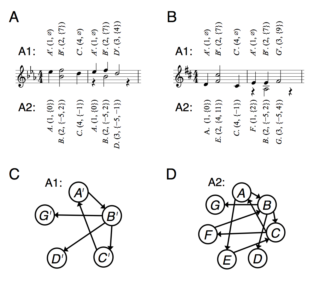
A Markov model consists of a state space, an initial distribution and a transition matrix (Norris, 1997). With the Racchmaninof-Oct2010 algorithm (Collins et al., 2016), we defined a state to consist of an ordered pair: beat of the bar on which a note/chord/rest occurs; spacing between MIDI notes occurring on that beat. Fig.s 1A and B contain two simplified “database pieces”, with the states according to this definition shown above the staves and prefaced with “A1”. For example, the chord in bar 1 of Fig. 1A, consisting of B♭4 and F5, begins on beat 2 and has a MIDI note spacing of 7 semitones, so is represented by the state \((2, \{7\})\), which happens to be labelled \(B^\prime\). The same beat-spacing state occurs in bar 2 beat 2 of Fig. 1A, bar 1 beat 2 of Fig. 1B and bar 2 beat 2 also. The transition matrix for these database pieces can be represented by the graph shown in Fig. 1C, with arrows indicating possible state-to-state transitions. The probabilities of these transitions can be defined according to the empirical likelihoods observed across multiple database pieces. With Racchmaninof-Oct2010, the definition of MIDI spacing for a lone note is the empty set, \(\emptyset\) and the definition of MIDI spacing for a rest is a special “rest” symbol (not featured in this example). When notes overlap in time, as in bar 2 beats 2–3 of Fig. 1A, we adhere to Pardo & Birmingham’s (2002) definitions of partition point and minimal segment to guide our analysis of simultaneously sounding (but not necessarily simultaneously beginning or simultaneously ending) pitch content.
With the Racchmaninof-Jun2015 algorithm, we change the definition of a state to consist of a slightly different ordered pair: beat of the bar on which a note/chord/rest occurs (same as before); MIDI notes occurring on that beat, relative to the global tonic (different to before). In the two simplified “database pieces” of Figs. 1A and B, states according to this new definition are shown below the staves and prefaced with “A2”. For example, the chord in bar 1 of Fig. 1A, consisting of B♭4 and F5, begins on beat 2, has a lower note occurring 5 semitones below the global tonic of E♭5 and a higher note occurring 2 semitones above the global tonic, so is represented by the state \((2, \{–5, 2\})\), which happens to be labelled \(B\). The same beat-relative-MIDI state occurs in bar 2 beat 2 of Fig. 1A and in bar 2 beat 2 of Fig. 1B. The corresponding transition matrix for these database pieces can be represented by the graph shown in Fig. 1D, with arrows indicating possible transitions as before and the probabilities of these transitions being defined similarly according to the empirical likelihoods observed across multiple database pieces. As with Racchmaninof-Oct2010, rests are encoded with a special “rest” symbol.
An advantage of the beat-spacing state space (Racchmaninof-Oct2010) over the beat-relative-MIDI state space (Racchmaninof-Jun2015) is that the former is smaller, leading to a less sparse transition matrix. There are fewer states in Fig. 1C compared with Fig. 1D and this is true of beat-spacing versus beat-relative-MIDI state spaces in general. In Collins et al. (2016), this was our main reason for using the beat-spacing state space for Racchmaninof-Oct2010, rather than the beat-relative-MIDI state space. Having seen how prone Cope’s EMI – which according to Cope (2005, p. 89) has a state space very similar to the beat-relative-MIDI definition – was to copying long segments of original material, we opted for the less sparse beat-spacing state space, where the chances of copying long segments of originals would be reduced.
A disadvantage of the beat-spacing state space is that it can generate tonally obscure material. To illustrate the potential for this eventuality, consider that in the A1 state sequence of Fig. 1D, there are two instances of the state \((2, \{7\})\), one in bar 1 beat 2 and another in bar 2 beat 2. The tonal function of these two chords is different, but they are analysed as the same state. When material is generated using a beat-spacing state space, MIDI note spacings need to be converted back into actual MIDI notes. One way in which this can be achieved is by using an initial seed MIDI note, plus information about the originally analysed notes, retained in a so-called “context”. Specifically, the interval in semitones between the lowest note of the current chord and preceding chord from the original context can be added to the seed note to get an actual MIDI note for the lowest note of the current chord and then the MIDI note spacing(s) is (are) added to this to get the higher note(s). From one note/chord to the next, there are intervallic relationships and voice-leading as evident in the database pieces, but beyond neighbouring notes/chords, such stylistic coherence is not guaranteed. In Collins et al. (2016), we introduced several constraints that were checked during the generation process (to do with pitch range and measuring the expectancy levels associated with different pitch combinations), in an effort to gain control over the level of tonal obscurity at any given point. According to the listening study results, we could not find a compromise between setting these constraints such that the output passages were stylistically successful and generating material within reasonable runtimes. In the current paper, therefore, we leave behind the beat-spacing state space in favour of exploring the beat-relative-MIDI state space.
To generate material with a state space and transition matrix such as that represented in Fig. 1D, all that is required is an initial distribution containing the likelihoods of possible first states (often constructed by recording the states that begin each database piece) and some pseudo-random numbers. The first pseudo-random number is used to select a new initial state, \(X_1\). The row of the transition matrix corresponding to \(X_1\) contains the likelihoods of possible next states, and the next pseudo-random number is used to select among these, producing a new next state \(X_2\). The row of the transition matrix corresponding to \(X_2\) contains the likelihoods of possible next states and the next pseudo-random number is used to select among these, producing a new next state \(X_3\) and so on, producing a generated state sequence \(X_1, X_2, X_3, ...\).
It is important to recognise that the state sequence \(X_1, X_2, X_3, ...\) consists of beat-relative-MIDI events, not the (ontime, MIDI note, duration)-triples that might be considered the minimum requirement for having generated music.(2) To get the ontimes from these states, we can assign ontime zero to \(X_1\) if \(X_1\) occurs on beat 1. If it occurs on some other beat, then we begin with an anacrusis corresponding to that amount. Inductively, if \(X_i\) begins on beat \(b\), has been assigned ontime \(x\) and \(X_{i + 1}\) begins on beat \(b^\prime > b\), then state \(X_{i + 1}\) is assigned ontime \(x + (b^\prime – b)\). If \(b^\prime \leq b\), because \(X_{i + 1}\) crosses a new bar line, then it is assigned ontime \(x + (b^\prime – b) + c\), where \(c\) is the number of crotchet beats per bar. To get the MIDI notes from relative MIDI notes, we select an original piece in the target style and calculate the MIDI note number of its tonic pitch class that is closest to the mean MIDI note number of the whole piece, denoted by \(m\). If \(X_i\) contains the relative MIDI notes \(m_1, m_2,..., m_k\), then the actual MIDI notes will be \(m_1 + m,\ m_2 + m,...,\ m_k + m\). To generate notes with actual and possibly different durations (e.g., giving rise to possibly overlapping notes), we make use of information about the analysed notes, retained in the context variable alongside the state (Collins et al., 2016). For example, for a relative MIDI note \(m_j\) in generated state \(X_i\), we can trace whether in its original context, \(m_j\) ended when \(X_i\) ended, or if it was held over into the next state. If it ended when \(X_i\) ended, then its duration will last up until but not beyond the ontime of \(X_{i + 1}\) in the generated sequence. Otherwise, if \(m_j\) is present in \(X_{i + 1}\) also, it could be sustained beyond the ontime of \(X_{i + 1}\) and, depending on membership of subsequent states, across several more generated states. In this way, the pseudo-randomly generated state sequence \(X_1, X_2, X_3,...\) can be converted to (ontime, MIDI note, duration)-triples and then to MIDI files, MusicXML files, etc.
While the example in Fig. 1 concerns which states proceed which, it is also possible to conduct an analysis of which states precede which, creating a “backwards” transition matrix and final (instead of initial) distribution (by recording the states that end each database piece). We discuss the musical utility of such an analysis in the next-but-one subsection on phrasal structure.
Our Racchmaninof algorithm is designed with the aim that each generated passage inherits the abstract, long-term repetitive structure of a preselected, original template piece/excerpt. We use a pattern discovery algorithm called SIACT (Collins, Thurlow, Laney, Willis, & Garthwaite, 2010), which is capable of automatically extracting the boxed repetitions shown in Figs. 2A and 3A. A point-set representation, with one dimension for ontime and a second for MIDI note, is the input to the algorithm, which searches exhaustively for so-called maximal translatable patterns (MTP, Meredith, Lemstrom & Wiggins, 2002). An MTP is a set of points that occurs at least once more in the point set under a single, nonzero, fixed translation vector. For example, the notes that are bound by the red dashed line in bars 1–5 of Fig. 2A and labelled \(P_{1,1}\) repeat in bars 6–10, labelled \(P_{1,2}\). There is a corresponding set of points in the point-set representation of this hymn that occur again under a translation of (20, 0), where 20 is 20 crotchet beats (or 5 bars later in common time) and 0 is 0 MIDI notes higher/lower than the original occurrence. The set occurring under this translation would be called the MTP of the vector \(\mathbf{v} = (20, 0)\). The output of the algorithms described by Meredith et al. (2002) is filtered according to several gestalt-like, perceptually validated steps, to produce the results shown in Figs. 2A and 3A (Collins et al., 2010). One attractive aspect of the point-set approach is that it supports the discovery of nested patterns. For instance, once in Fig. 2A, \(P_{2,1}\) repeats as \(P_{2,2}\), as a natural consequence of \(P_{1,1}\) repeating as \(P_{1,2}\). On the second repeat (third occurrence), however, \(P_{2,3}\) appears independently of the earlier five-bar pattern. These long-term dependencies and nested structures seem to be the kind to which Widmer (2016) refers.


In order that the Racchmaninof algorithm’s output inherits such abstract, long-term repetitive structures, it is important to ensure that material is generated and put in place first for the time window corresponding to the most nested discovered pattern. In Figs. 2A and 2B, \(P_{2,1}\) and \(P_{2,2}\) are equally most nested, each being subsets of one larger discovered pattern (\(P_{1,1}\) and \(P_{1,2}\) respectively). Therefore, using the Markov model described above, Racchmaninof would generate material for the ontime interval [13, 20), corresponding to bar 4 beat 2 up to and including bar 5. Using 45 original four-part hymns by Bach as database pieces, not including the piece used as a template in Fig. 2A, we constructed a Markov model and used Racchmaninof to generate material for the interval [13, 20).(3) The output is shown bound by the solid blue box and labelled \(P_{2,1}\) in Fig. 2B. It is “copied and pasted” to the ontime interval [33, 40), as indicated by the solid blue box labelled \(P_{2,2}\) and again to the ontime interval [71, 77) – the solid blue box labelled \(P_{2,3}\). Next, the Racchmaninof algorithm generates material for the next most nested pattern (\(P_{1,1}\) or \(P_{1,2}\)). As some of the ontime interval [0, 20) contains material already, it uses the state at ontime 13 as a constraint (more details on which in the next subsection), and fills the remaining time interval [0, 13). The generated output is copied and pasted to the ontime interval [20, 33). Finally, Racchmaninof generates output for the remaining ontime interval, [40, 71). It does not generate material for intervals under one bar in length, so the final two beats of the generated passage contain a rest. The passage shown in Fig. 3A is generated in an analogous fashion, but the Markov model is constructed using different database pieces (mazurkas by Chopin) and there are more discovered patterns to inherit in this particular example.(4)
As mentioned at the end of the subsection introducing Markov models, it is possible to Markov-generate backwards as well as forwards. From a musical point of view, forwards- and backwards-running material can be joined with the aim of achieving output that is perceived as having a beginning, middle and end (in other words, phrasal structure, Cope, 2005; Collins et al., 2016). For instance, in Fig. 2B, material will have been generated to cover the ontime interval [38, 71], corresponding to bar 10 beat 3 through to bar 18 beat 4. This material will have resulted from generating three candidate passages forwards to fill the interval [38, 54], three candidate passages backwards to fill the interval [54, 71] and then using three joining techniques to determine the events at ontime 54 (bar 14 beat 1). In this instance, the join works very well, with good voice-leading approaching and proceeding from bar 14 beat 1. On other occasions the join is less successful, leading to poor voice-leading or unusual chord superpositions (see Fig. 2B, bar 5 beat 1).
If state \(X_{i – 1}\) from a forwards-generated passage and state \(X_{i + 1}\) from a backwards-generated passage are to be joined, a set \(A\) of forwards continuations from state \(X_{i – 1}\) is determined, as is a set \(B\) of backwards continuations from state \(X_{i + 1}\) and a random selection is made from their intersection \(A \cap B\), if it is nonempty.(5) Bar 14 beat 1 of Fig. 2B is an example of one such join. If \(A \cap B\) is empty, however, then our Racchmaninof-Jun2015 algorithm reverts to the joining methods of the earlier Racchmaninof-Oct2010 algorith (Collins et al., 2016), which include overwriting state \(X_{i + 1}\) with some forwards continuation of \(X_{i – 1}\), overwriting state \(X_{i – 1}\) with some backwards continuation of state \(X_{i + 1}\), or the superposition of states. Superposition is the method behind the material at bar 5 beat 1 of Fig. 2B.
Sometimes we will want the opening note/chord of an arbitrary ontime interval \((a, b)\) to sound like it comes from the very beginning of a piece (e.g., if \(a = 0\)). On other occasions (if \(a > 0\)), it is desirable that the opening note/chord sounds appropriate as the beginning of a phrase but not necessarily the beginning of the whole piece. The same reasoning applies to the ending of a piece/phrase. So as well as constructing “external” distributions from the initial and final notes/chords in the database pieces, we also construct “internal” distributions using the fermatas and phrase markings in the digital encodings. It is our premise that with these four initial distributions and two transition matrices (one forwards and one backwards), material having phrasal structure may be generated.
As well as stipulating that no more than four consecutive generated states may come from the same original corpus piece and imposing this constraint during the generation process, we also conducted a post-generation analysis of Racchmaninof’s output, to determine whether copying occurred anyway (e.g., because if a generated passage’s sources are \(... X, X, X, X, Y, X, X, X, X,...\), which would satisfy the simple four consecutive sources constraint, this might still be perceived as copying source \(X\)) and to investigate the originality/creativity of Racchmaninof’s output more generally. The following section is devoted to describing the results of this originality/creativity analysis.
Defining a measure of originality or creativity is not straightforward, but in the first instance we can compare one or more bars of a generated passage with the same number of bars from an original piece and quantify the similarity of these two excerpts by calculating the number of (ontime, MIDI note)-pairs they have in common, up to transposition, divided by the maximum number of common pairs if they were identical or exact transpositions of one another. Letting \(P\) denote the (ontime, MIDI note)-pairs of \(n\) bars of music from a corpus piece and \(Q\) denote the (ontime, MIDI note)-pairs of \(n\) bars from a generated passage, this quantification of similarity, known as the cardinality score, is given by the formula \(s(P, Q) = (P \cap Q)/\max\{|P|, |Q|\}\). To achieve transpositional invariance, the formula is calculated for all possible transpositions of \(Q\) such that \(P\) and \(Q\) have at least one note in common, then the maximum calculated value is taken to be the cardinality score. We adapt this concept from work by Ukkonen, Lemström & Mäkinen (2003) on pattern matching symbolic music queries against a corpus.
A worked example may be helpful. Letting \(P\) denote the (ontime, MIDI note)-pairs of the notes belonging to bar 1 of Fig. 3A, there are eleven elements in \(P\). If you count twelve, notice that the ontime of the piece’s opening A4 precedes bar 1 and so is not an element of \(P\). Letting \(Q\) denote the (ontime, MIDI note)-pairs of the notes belonging to bar 6 of Fig. 3A, there are ten elements in \(Q\). The denominator of the cardinality score is \(\max\{|P|, |Q|\} = \max\{11, 10\} = 11\). Considering how \(P\) might be transposed so that as many as possible of its (ontime, MIDI note)-pairs coincide with those of \(Q\), we see the transposition of five semitones up (a perfect fourth) provides this maximal coincidence, transposing (1) the D2 of bar 1 to the G2 of bar 6, (2) the D3 of bar 1 beat 2 to the G3 of bar 6 beat 2, (3) the A3 of bar 1 beat 2 to the D4 of bar 6 beat 2, (4) the D3 of bar 1 beat 3 to the G3 of bar 6 beat 3 and (5) the A3 of bar 1 beat 3 to the D4 of bar 6 beat 3. The numerator of the cardinality score is \(P \cap Q = 5\), giving a cardinality score of \(s(P, Q) = 5/11 \approx .45\). In an implementation, this maximal transposition and the amount of coincidence in which it results can be determined by calculating the vector difference between each \(\mathbf{p} \in P\) and \(\mathbf{q} \in P\), counting how often each difference vector occurs and returning the maximal frequency.
For each generated passage and each original corpus piece, we calculated cardinality scores of queries of length \(n = 1\) bar and recorded the maximum observed cardinality score. These maximum query similarity to corpus scores are plotted as the solid blue line in Fig. 4 for the generated passage from Fig. 2B. Maximum observed cardinality scores were also recorded for queries of length \(n = 2\) bars (dashed blue line in Fig. 4). In general, as the query’s bar length is increased, the maximum query similarity to corpus should decrease: if bar \(y\) of the generated passage is very similar to bar \(y^\prime\) of an original piece, then the maximum cardinality score for query length \(n = 1\) bar will be high; if bar \(y + 1\) in the generated passage deviates from bar \(y^\prime + 1\) of the original piece, then when the query length is increased to \(n = 2\) bars, the generated and original-piece queries, now encompassing bars \(y\) to \(y + 1\) and \(y^\prime\) to \(y^\prime + 1\) respectively, are no longer so similar and the cardinality score will decrease compared with \(n = 1\). If, however, the cardinality score stays high as \(n\) increases, this is an indication that the generated passage borrows too heavily from an original corpus piece.
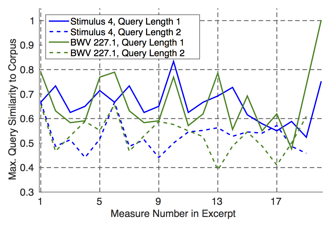
When a passage is generated using corpus piece \(X\) as a template, material from \(X\) is not included in any of the initial distributions or transition matrices (another step to avoid copying originals). Therefore, we can also conduct a creativity/originality analysis for the original template piece \(X,\) to see whether the generated passage is about as creative or original as the template and to investigate general issues of creativity/originality across different corpora (e.g., are Chopin mazurkas generally more distinct from one another than are Bach hymns?). For the template piece from Fig. 2A, the maximum query similarity to corpus scores are plotted as the solid (\(n = 1\) bar) and dashed (\(n = 2\) bars) green lines in Fig. 4. Comparing the solid lines with one another and the dashed lines with one another, it can be seen that the values are similar and that in terms of whole-bar copying, the generated passage is no less original or creative an instance of a Bach four-part hymn than the original template piece.
Previous analysis (Collins et al., 2016) of Cope’s EMI output (1996) can be used as a benchmark for copying thresholds (i.e., “how much copying is too much?”). There, the cardinality score remained at .63 as \(n\) increased to twenty bars of music. From Fig. 4, it can be seen that as early as \(n = 2\), there are only two maximum cardinality scores exceeding .6 for the generated passage. As \(n\) increases further, these maxima fall easily below the threshold observed in EMI’s Mazurka no. 4 in E minor (Cope, 1996). Therefore, we can assert that the output of Racchmaninof guards against plagiarism of originals in ways that EMI does not. It may be helpful to end this whole section with some further remarks concerning how the current research extends beyond that of Cope (1996, 2001, 2005): unlike with EMI, the full source code for Racchmaninof-Jun2015 will be made available, making it possible to replicate the generation of those passages shown above in Figs. 2A and 3A, as well as those included below with the description of the listening study.(6) This is in keeping with the general approach of releasing source code to members of the academic community, as was done for Racchmaninof-Oct2010 (Collins, 2011); while Cope (2005) and Hofstadter (in Cope, 2001) only provide quite broad descriptions of Markov model construction and templagiarism, we have attempted to be more explicit and provide concrete examples and walk-throughs; we have evaluated (Collins et al., 2016) and are about to describe a new evaluation of our algorithms in a listening study, which we and others contend is the best-practice approach to assessing a model of stylistic composition (Pearce et al., 2002; Pearce & Wiggins, 2001; Pearce & Wiggins, 2007).
This section describes a listening study that was designed to address the following topics and questions:
Stylistic success. How do Bach hymns generated by our algorithm Racchmaninof-Jun2015 compare in terms of stylistic success to original four-part hymns by Bach? How do Chopin mazurkas generated by Racchmaninof-Jun2015 compare in terms of stylistic success to original Chopin mazurkas, and how do our algorithms Racchmaninof-Oct2010 and Racchmaninof-Jun2015 compare to each other?
Distinguishing. Can participants distinguish reliably (i.e., significantly better than chance) between the human-composed and computer-generated stimuli?
Reliability. Is there a significant level of inter-participant reliability, in terms of the stylistic success ratings for each stimulus?
Participants were recruited from the following email lists: the Society for Music Theory, ISMIR Community, Music and Science, and the Society for Music Perception and Cognition. We limited circulation to these lists in order to try to target relatively expert listeners. Participants were directed to a website introducing the listening study, the target styles and the types of questions that they would go on to answer after listening to each music stimulus. Participants were told that providing a full data set would entitle them to be entered into a draw to win a £50 Amazon voucher. They gave informed consent before proceeding to the first block of the listening study, Bach hymns, which took approximately 20 minutes to complete and which was followed by a second slightly longer block on Chopin mazurkas. Ratings of stylistic success were gathered on a scale 1–7 (1 = low, 7 = high). We also collected ratings of aesthetic appeal (how much a participant enjoyed a given stimulus) according to the same scale. A further question asked participants to distinguish between whether the stimulus played was a human composition or computer generated. There were two open-ended text boxes – one for comments on the stylistic success rating in particular and a second for any other comments about the stimulus. The general design of the listening study is in keeping with the adaption of the CAT (Amabile, 1996; Collins et al., 2016; Pearce & Wiggins, 2007).
The new computer-generated stimuli were all generated by algorithm Racchmaninof-Jun2015 using the Bach and Chopin corpora as in the previous section. We set a constraint that during the generation process, no more than four consecutive states could come from the same original source piece. Six computer-generated stimuli from algorithm Racchmaninof-Oct2010 (Collins et al., 2016) were included, in an effort to assess quantitatively any improvements between Racchmaninof-Oct2010 and Racchmaninof-Jun2015. Within Bach hymn and Chopin mazurka blocks, the presentation order of stimuli was shuffled for each participant in order to avoid ordering effects. The stimulus details are as follows:
| No. | Audio | Details |
|---|---|---|
| 1 | BWV 411/R 246 | |
| 2 | Generated passage (Racchmaninof-Jun2015) | |
| 3 | BWV 350/R 360 | |
| 4 | Generated passage (Racchmaninof-Jun2015) | |
| 5 | BWV 325/R 235 | |
| 6 | Generated passage (Racchmaninof-Jun2015) | |
| 7 | BWV 180.7/R 22, see also Fig. 2A | |
| 8 | Generated passage (Racchmaninof-Jun2015), see also Fig. 2B | |
| 9 | BWV 407/R 202 | |
| 10 | Generated passage (Racchmaninof-Jun2015) | |
| 11 | BWV 227.1/R 263 | |
| 12 | Generated passage (Racchmaninof-Jun2015) | |
| 13 | Chopin op. 24 no. 1 bb. 1–16, see also Fig. 3A | |
| 14 | Generated passage (Racchmaninof-Jun2015), see also Fig. 3B | |
| 15 | Chopin op. 56 no. 2 bb. 1–16 | |
| 16 | Generated passage (Racchmaninof-Jun2015) | |
| 17 | Chopin op. 7 no. 2 bb. 1–16 | |
| 18 | Generated passage (Racchmaninof-Jun2015) | |
| 19 | Chopin op. 33 no. 4 bb. 1–16 | |
| 20 | Generated passage (Racchmaninof-Jun2015) | |
| 21 | Chopin op. 7 no. 4 bb. 1–16 | |
| 22 | Generated passage (Racchmaninof-Jun2015) | |
| 23 | Chopin op. 24 no. 3 bb. 1–16 | |
| 24 | Generated passage (Racchmaninof-Jun2015) | |
| 25 | Generated passage (Racchmaninof-Oct2010) | |
| 26 | Generated passage (Racchmaninof-Oct2010) | |
| 27 | Generated passage (Racchmaninof-Oct2010) | |
| 28 | Generated passage (Racchmaninof-Oct2010) | |
| 29 | Generated passage (Racchmaninof-Oct2010) | |
| 30 | Generated passage (Racchmaninof-Oct2010) |
51 people registered to participate. Three provided nonsense contact information and did not submit data. A further fourteen provided sensible contact and musical background information but did not submit data. Of the remaining 34 participants, nine recognised one or more of the excerpts from original Bach hymns, providing comments along the lines of “It is by Bach, I recognise it as one of the chorale tunes”. For the following quantitative analyses, we put these participants’ data to one side, because answering on the basis of recognition confers an unfair advantage and/or could bias responses. The analysis proceeds using data from the remaining 25 participants.
On inspecting distributions of participants’ years of formal musical training, regularity of playing a musical instrument or singing and regularity of concert attendance, we saw no grounds for forming two groups of participants (i.e., by median-splitting the participants into one less and one more expert group). There was bimodality evident in some of these distributions, but it was not always due to the same subgroup of participants. So we proceed with one group of participant data.
Distinguishing. Five out of 25 participants scored significantly better than chance when distinguishing between original Bach hymn excerpts and computer-generated passages.(7) Four participants scored ten out of twelve, one scored eleven, but no one scored twelve. These results suggest that the Racchmaninof-Jun2015 algorithm produces passages in the style of Bach hymns that are very difficult to distinguish from the originals, even for participants with a mean of 8.56 years of formal musical training and mode “daily/weekly” regularity of playing an instrument or singing.
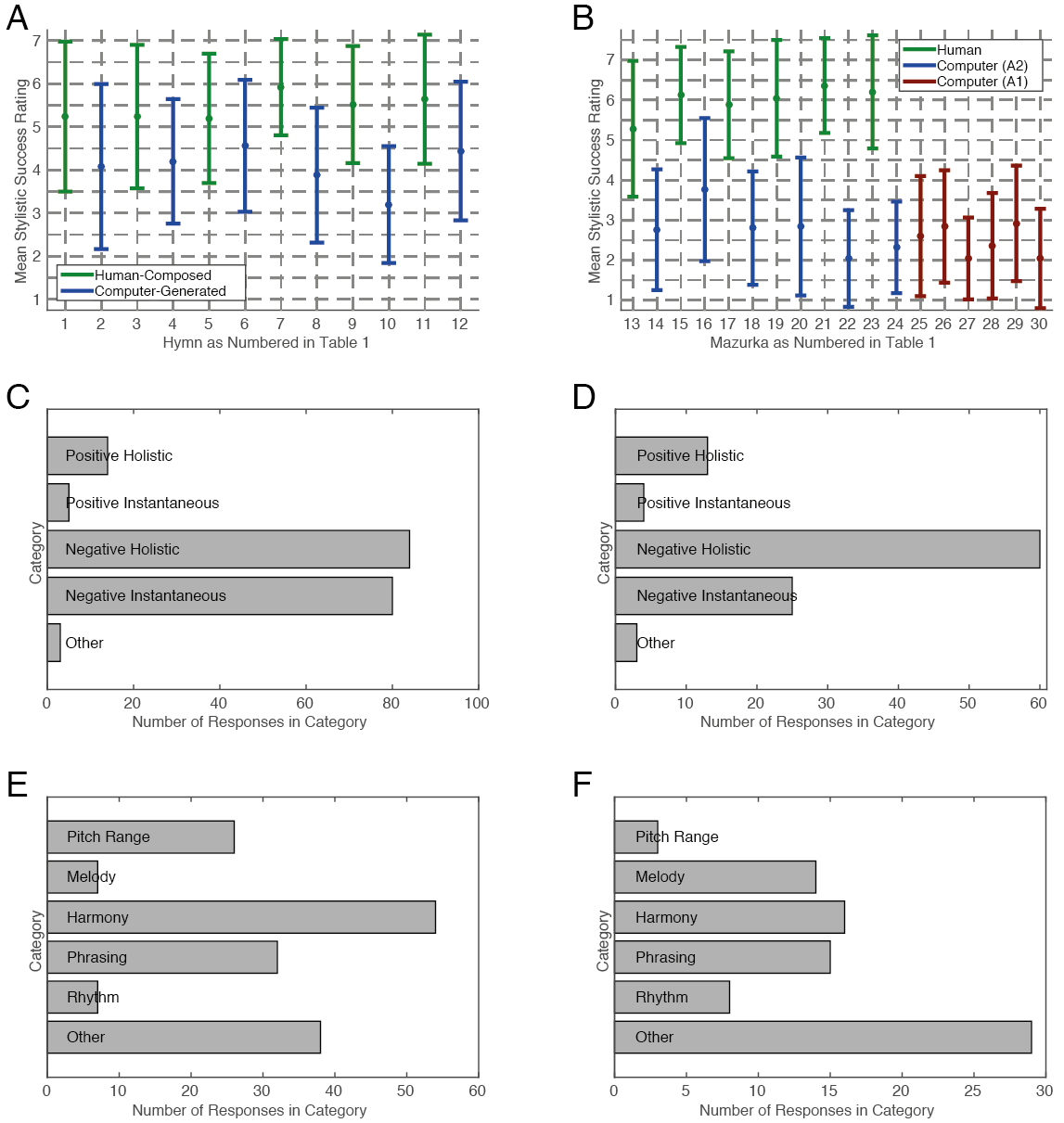
Stylistic success. We calculated the mean stylistic success ratings across the 25 participants for each of the twelve excerpts (see Fig. 5A). Calculating means across participants was justified by a significant value of Kendall’s coefficient of concordance for the stylistic success ratings \((W = .262, \chi^2(11) = 72, p < .001).\) We then tested whether the mean ratings for the original Bach hymn excerpts were significantly higher than those for the computer-generated passages by conducting a two-sample \(t\)-test. The difference was significant (\(t(10) = 6.07,\ p < .001),\) suggesting that the original Bach hymn excerpts are more successful stylistically than the computer-generated passages. Therefore, while only five out of 25 participants were able to distinguish reliably between human-composed and computer-generated Bach hymns, it seems their stylistic success ratings were more effective discriminators.
As a continuation of the Bach hymn block of the study, 51 people were also registered to participate in the Chopin mazurka block. Therefore, the same three provided nonsense contact information and did not submit data. One submitted data but it comprised uniform stylistic success and aesthetic pleasure ratings of 4 and so was removed. In addition to the fourteen who provided sensible contact and musical background information but did not submit Bach data, two participants submitted Bach data but did not submit Chopin data. They had spent longer than the allotted time on the Bach block of the study and so probably did not wish to listen to further excerpts in the style of (or by) Chopin. Of the remaining 31 participants, six provided comments indicating recognition of one or more of the original Chopin mazurka excerpts. So again, for the following quantitative analyses we put these participants’ data to one side, and the analysis proceeds using data from the remaining 25 participants. With a large overlap between these participants and those from the Bach block of the study, the musical background information was mostly unchanged.
Similar to the Bach block, the Chopin block comprised six original mazurka excerpts and six generated by Racchmaninof-Jun2015. We had access to a further six passages generated by Racchmaninof-Oct2010 (Collins et al., 2016) and so included these too – the aim being to assess quantitatively the improvement between Racchmaninof-Oct2010’s output and that of Racchmaninof-Jun2015.
Distinguishing. Sixteen out of 25 participants scored significantly better than chance when distinguishing between original Chopin mazurka excerpts and passages generated by Racchmaninof-Jun2015. Seven participants scored ten out of twelve, three scored eleven and six scored twelve. These results suggest that the Racchmaninof-Jun2015 algorithm produces passages in the style of Chopin mazurkas that are relatively easy to distinguish from the originals for participants with a mean of 6.84 years of formal musical training and mode “daily” regularity of playing an instrument or singing.
Stylistic success. We calculated the mean stylistic success ratings across the 25 participants for the six original mazurka excerpts and Racchmaninof-Jun2015 output passages (see Fig. 5B). Calculating means across participants was justified by a significant value of Kendall’s coefficient of concordance for the stylistic success ratings \((W = .674, \chi^2(11) = 185, p < .001).\) It is worth noting that the value of Kendall’s \(W\) alone cannot be used to make inferences about the success or otherwise of a particular algorithm’s output. We are using it only to justify the taking of means, which are then tested to make inferences about comparative stylistic success. In particular, the value of \(W\) being higher for the Chopin block (\(W = .674\)) than it was for the Bach block (\(W = .262\)) does not imply that the algorithm was better or worse at generating Bach-style passages than Chopin-style passages. After taking means, we then tested whether the mean ratings for the original Chopin mazurka excerpts were significantly higher than those for the computer-generated passages, by conducting a two-sample \(t\)-test. The difference was significant (\(t(10) = 11.32,\ p < .001),\) suggesting that the original Chopin mazurka excerpts are more successful stylistically than the computer-generated passages. The value of \(t\) being higher for the Chopin block (\(t = 11.32\)) than it was for the Bach block (\(t = 6.07\)) does suggest that Racchmaninof-Jun2015 is better at generating Bach-style passages than Chopin-style passages – a finding that echoes participants’ ability to distinguish computer-generated and original Chopin mazurkas with ease, compared to computer-generated and original Bach hymns.
Improvement between Racchmaninof-Oct2010 and Racchmaninof-Jun2015. The stylistic success ratings for passages generated by Racchmaninof-Jun2015 and Racchmaninof-Oct2010 (see Fig. 5B) indicate a significant improvement for Racchmaninof-Jun2015’s output compared with that of Racchmaninof-Oct2010. We did not calculate mean stylistic success ratings across the 25 participants for these passages, because Kendall’s coefficient of concordance was less than a quarter of that observed directly above (\(W = .158\) opposed to \(W = .674\)) and just over half of that observed for the Bach excerpts (\(W = .262\)).(8) Instead, we tested whether the unaveraged ratings for passages generated by Racchmaninof-Jun2015 were significantly higher than those of Racchmaninof-Oct2010. The difference was significant (\(t(298) = 1.70,\ p < .05)\), suggesting that the passages generated by Racchmaninof-Jun2015 are more stylistically successful as Chopin mazurkas than those generated by Racchmaninof-Oct2010.
In terms of participants’ ability to distinguish correctly that Racchmaninof-Jun2015 and Racchmaninof-Oct2010 output was computer-generated, the mean distinguishing score for Racchmaninof-Jun2015 was marginally lower (5.28/6) than that of Racchmaninof-Oct2010 (5.6/6), indicating it may have been harder to tell that Racchmaninof-Jun2015’s output was not real Chopin than it was to tell Racchmaninof-Oct2010’s output was not real Chopin, but this is not a significant difference.
We analysed all comments that participants made about the computer-generated passages (see Fig. 5C and 5E for Bach hymns and Fig. 5D and 5F for Chopin mazurkas), including those comments from participants whose data was excluded from previous analyses due to explicitly recognising certain excerpts. Comments were categorised into “positive holistic” (a generally positive remark about an excerpt), “positive instantaneous” (a positive remark about a specific moment in an excerpt), “negative holistic”, “negative instantaneous” and “other” (e.g., a statement of fact that was neither positive nor negative). The results of this categorisation process are shown in Figs. 5C and 5D. Then, focusing on negative comments only, we further categorised the comments into six categories that have been used previously (Collins et al., 2016; Pearce & Wiggins, 2007): “pitch range”, “melody”, “harmony”, “phrasing”, “rhythm” and “other”. The corresponding frequency counts are shown in Fig. 5E for Bach hymns and Fig. 5F for Chopin mazurkas. It can be seen by comparing Figs. 5C and 5D that generally participants made more comments about the generated Bach hymns than they did about generated Chopin mazurkas. Participants were equally likely to make negative holistic and instantaneous comments about the Bach hymns, whereas the Chopin mazurkas tended to invite more negative holistic comments than other comment types. Ordering effects as well as participant backgrounds could be driving these differences – not just differences in Racchmaninof’s ability to generate Bach hymns versus Chopin mazurkas.
Some listeners made only holistic comments (a participant comments on generated chorale no. 8 from Tab. 1 that it “Had a couple of inconsistencies with the flow”), but most provided a mixture of instantaneous and holistic remarks. For examples of instantaneous remarks, a participant said of generated chorale no. 10 from Tab. 1, “Very few chorales start phrases with such long chord! … The change of register in the first phrase is too drastic … some NCTs [non-chord tones]”; another participant said of generated chorale no. 6 from Tab. 1, “Four seconds in, there is an awkward-sounding chromatic addition/secondary dominant on the final beat that sounds completely un-Bach like to me. That’s the moment that spoiled it for me”; another participant said of generated chorale no. 2 in Tab. 1, “Up until the last few notes it sounded real then it went wrong”. These comments suggest that a generated passage can be “90–95% successful”, but be “caught out” as computer-generated and/or given a low stylistic success rating due to a single moment. This has ramifications for future work, suggesting for instance that the joins between forwards- and backwards-generated material require more careful management, because an instantaneous shortcoming in joining two passages could make the difference between an overall high or low stylistic success rating.
So-called “other” remarks were the most numerous in the breakdown of negative comments on Chopin mazurkas (Fig. 5F). Most often, comments were categorised as such because they mentioned no dimension of music in particular, rather than mentioning some aspect not included in the list “pitch range”, “melody”, “harmony”, “phrasing”, “rhythm”. The following non-specific remark was quite typical, for instance: on mazurka no. 14 from Tab. 1, “I can hear derivatives of Chopin in this, but it doesn’t convince me”. Here, on the other hand, is a rarer comment that mentions an aspect of music not included in the list: on mazurka no. 18 from Tab. 1, “It was almost successful if it had not been for the staccato chords in the accompaniment”.
It seems from Figs. 5E and 5F that the phrasing of the Racchmaninof-Jun2015 algorithm still needs attention, but most often these comments related to unusual or unexpected pauses, so this might be addressed by fitting the note density of a generated passage to that of the template piece. It was encouraging to see comments that reflected listeners’ sensitivities to repetitive structure, even though the content of those repetitions may have caused them to question if they were listening to original Bach or Chopin excerpts: a participant said of generated mazurka no. 18 from Tab. 1 that “Its leap at 3s is funny. It repeats though, so I don’t know”.
With large multinational technology companies investing heavily in the simulation of human intelligence and creativity (e.g., Google’s scientific evaluation of a computational system capable of beating the best human players of the Chinese board game Go), it is notable that the simulation of musical creativity remains an elusive, open challenge (as evidenced by the same company’s recently announced Magenta project, which has the aim of using “machine learning to create compelling art and music”).(9) The task of listening “blind” to a given excerpt of music and forming judgments concerning its stylistic success and human/computational provenance appears to be very appealing, with the study described above attracting 51 participants. The appeal of such tasks and the ease with which they can be conducted online (while still being able to monitor participants’ engagement, e.g., through the use of timestamps) calls into question why more researchers are not evaluating their music-computational models rigorously via listening studies. The nature and ramifications of the simulation of musical creativity are as important – if not more – than those associated with simulation of board game play, so perhaps it is time we stopped accepting informal evaluations (“the quality of the output is high”) or even purely metric-based evaluations (“the quantity of the output as measured by this metric is high”), in favour of the scientific approaches proposed a decade or more ago (Amiable, 1996; Pearce & Wiggins, 2001; Pearce & Wiggins, 2007; Pearce, Meredith & Wiggins, 2002).
The Racchmaninof-Jun2015 algorithm has already had an unexpected impact outside the rather narrow field of generating entire stylistic passages. It has been used by music psychologists, for example, in order to generate stylistically coherent yet controllable material for melodic memory listening tests (Harrison, Collins & Müllensiefen, 2016). We would welcome its combination with other packages for creating music, such as OpenMusic. Upon request, the source code has been and will continue to be released to other academics under the GNU General Public License. We have not made the package completely open source (e.g., hosting on GitHub), in order to reduce the chances of unlicensed use in commercial music-generating applications.
The main result of the listening study is that the algorithm Racchmaninof-Jun2015 generates passages that are generally indistinguishable from original Bach hymns. These passages are complete musical textures, consisting of ontimes, pitches, durations and voice assignations – not reharmonizations of existing melodies. To our knowledge, Racchmaninof-Jun2015 is the first system capable of such a task. To the extent that long-term repetitive and phrasal structure contributes to the perceived stylistic success of an excerpt, this feat invites the conclusion that Racchmaninof-Jun2015 offers one effective method of addressing Widmer’s (2016) long-term dependency challenge. Widmer’s (2016) manifesto, including the observation that music is fundamentally non-Markovian, urges researchers to develop analytical and compositional models that take into account music’s long-term dependencies, including (but not limited to) its use of tonality, themes, repeated sections, harmonic rhythm and phrasing. The Racchmaninof algorithm nests a Markovian approach within processes designed to ensure that the generated material has both long-term repetitive and phrasal structure. In contrast to Widmer’s (2016) observation, our premise is that Markovian and non-Markovian approaches can be combined to achieve realistic models of music-analytic and music-compositional processes. We agree, however, that long-term dependency (or non-Markovian aspects) has been overlooked by music computing researchers in general and that this is where more attention and rigorous evaluation needs to be focused. It would perhaps be helpful if music computing researchers put their code to one side and attempted some of the long-standing stylistic composition tasks themselves. This would foster a deeper understanding and mastery of the long-term dependencies in music that such tasks demand and could lead to better computational models of these dependencies in future.
The achievement above, pertaining to generation of Bach hymns, should be tempered with another outcome of the study, which is that Racchmaninof’s generated passages in the style of Chopin mazurkas are easily distinguished from the originals, by approximately two thirds of listeners. It might be concluded reasonably from these findings that the computer generation of stylistically successful Chopin mazurkas is an inherently more difficult task than generation of stylistically successful Bach hymns. This conclusion is underlined further by the way in which Racchmaninof-Jun2015 grew out of modifications to Racchmaninof-Oct2010 (Collins et al., 2016) – a system designed specifically with the generation of Chopin mazurkas in mind. If an algorithm had been developed specifically with the generation of Bach hymns in mind and then its application to Chopin mazurkas had failed, it could be surmised that the developers had focused too narrowly on modelling characteristics of Bach hymns – characteristics that were irrelevant or counterproductive in the context of Chopin mazurkas. Racchmaninof-Jun2015, however, designed with the aim of Chopin mazurka generation, falls short in this regard, yet successfully generates Bach hymns.
This article includes the first description of attempts to improve joins between forwards- and backwards-generated material. In particular, if state \(X_{i – 1}\) from a forwards-generated passage and state \(X_{i + 1}\) from a backwards-generated passage are to be joined, a set \(A\) of forwards continuations from state \(X_{i – 1}\) is determined, as is a set \(B\) of backwards continuations from state \(X_{i + 1}\) and a random selection is made from their intersection \(A \cap B\), if it is nonempty. This method results in joins that have convincing voice-leading and that do not seem to attract negative stylistic comments from participants. Bar 14 beat 1 of Fig. 2B was mentioned above as one such join. If \(A \cap B\) is empty, however, then Racchmaninof-Jun2015 reverts to the joining methods of Racchmaninof-Oct2010 (Collins et al., 2016), which include overwriting state \(X_{i + 1}\) with some forwards continuation of \(X_{i – 1}\), overwriting state \(X_{i – 1}\) with some backwards continuation of state \(X_{i + 1}\), or the superposition of states. The superposition method especially causes some noticeably unsuccessful moments (e.g., see bar 5 beat 1 of Fig. 2B) and attracts negative stylistic comments from participants. So state superposition ought to be revised considerably in future work or dropped altogether.
While this suggested modification may seem slight, it could lead to substantial improvements in stylistic success ratings: we base this claim on a general observation that participants judge excerpts quite harshly, even if the stylistic transgression is relatively superficial or momentary. For instance, one participant gave excerpt N (a Bach hymn original) a stylistic success rating of two out of seven, commenting “In general, last chord of cadences lasts too long”. If a student had submitted this for a hymn composition task, then a mark of 29% (\(\approx 2/7\)) would be harsh, if the only perceived shortcoming was that phrase-ending chords were too long in duration.
The stylistic success of generated Chopin mazurkas might be improved by expanding and modifying the internal initial and final distributions. Currently, these are formed from marked phrase-opening and closing events in the scores, but only the first three internal phrase openings and last three internal phrase closings per piece (and fewer if Chopin happened to mark less than three). With the hymns, on the other hand, Bach marked fermata in keeping with the texts and there are typically more than three fermatas per piece. Consequently, the internal initial and final distributions for the Bach model contain more states, which may increase the probability of generating stylistically successful material.
A more general observed shortcoming of the generated mazurka passages was that they lacked “melodic character”. Further work is required to determine whether such character can be distilled into calculable musical features. For example, it could be said that the melody in Fig. 3B “lacks character” compared with the melody in Fig. 3A, but according to which features do the two melodies differ, and of these features, which are implicated regularly in melodies possessing or lacking character? One obvious candidate feature is intervallic leaps, with the melody in Fig. 3B containing many more than the melody in Fig. 3A. But is number (or proportion) of intervallic leaps a reliable, significant predictor of lacking melodic character, or a feature that could account for different ratings for these two excerpts only? Previous work has identified many potentially useful symbolic features (Collins et al., 2016; Pearce & Wiggins, 2007; Madsen & Widmer, 2007; Müllensiefen, 2009) and shown how they might be combined into regressions on stylistic success ratings so as to test their general predictive power (Collins, 2011; Pearce & Wiggins, 2007). Such an analysis could be a topic of future work and may lead to the definition of new constraints to be applied during the generation process. It could be that different constraints and/or different parameter values associated with those constraints will apply to different target styles and that this is how we can build further on the achievements described within this article – extending our approach from stylistically successful generation of Bach hymns to other composers and genres of music.